[av_one_full first min_height=” vertical_alignment=” space=” custom_margin=” margin=’0px’ padding=’0px’ border=” border_color=” radius=’0px’ background_color=” src=” background_position=’top left’ background_repeat=’no-repeat’ animation=”]
[av_textblock size=’35’ font_color=” color=” av-medium-font-size=” av-small-font-size=” av-mini-font-size=” admin_preview_bg=”]
Sojourner Generation 4
Summary Blog Post
[/av_textblock]
[av_hr class=’default’ height=’50’ shadow=’no-shadow’ position=’center’ custom_border=’av-border-thin’ custom_width=’50px’ custom_border_color=” custom_margin_top=’30px’ custom_margin_bottom=’30px’ icon_select=’yes’ custom_icon_color=” icon=’ue808′ font=’entypo-fontello’ admin_preview_bg=”]
[av_textblock size=” font_color=’custom’ color=’#bfbfbf’ av-medium-font-size=” av-small-font-size=” av-mini-font-size=” admin_preview_bg=”]
Authors:
Robert Francis Pearson (Project Manager), David Garcia (MST Engineer), Alex Dalton (EC Engineer)
Verification:Robert Francis Pearson
Approval:Robert Francis Pearson
Table of Contents
[/av_textblock]
[av_hr class=’short’ height=’50’ shadow=’no-shadow’ position=’left’ custom_border=’av-border-thin’ custom_width=’50px’ custom_border_color=” custom_margin_top=’30px’ custom_margin_bottom=’30px’ icon_select=’yes’ custom_icon_color=” icon=’ue808′ font=’entypo-fontello’ admin_preview_bg=”]
[av_textblock size=” font_color=” color=”]
[/av_textblock]
[av_heading tag=’h1′ padding=’10’ heading=’Executive Summary’ color=” style=” custom_font=” size=” subheading_active=” subheading_size=’15’ custom_class=” admin_preview_bg=” av-desktop-hide=” av-medium-hide=” av-small-hide=” av-mini-hide=” av-medium-font-size-title=” av-small-font-size-title=” av-mini-font-size-title=” av-medium-font-size=” av-small-font-size=” av-mini-font-size=”][/av_heading]
[av_textblock size=” font_color=” color=” av-medium-font-size=” av-small-font-size=” av-mini-font-size=” admin_preview_bg=”]
Space the final frontier. All from the joy of your home. Meet Sojourner a smaller, lovable version of the JPL Pathfinder. This robot implements a novel method of monitoring its own speed to adapt and overcome its environment. To perform this task, Sojourner implements the latest in sensorless rpm encoding through monitoring commutator noise and back EMF.
[/av_textblock]
[av_heading tag=’h2′ padding=’10’ heading=’Program and Project Objectives’ color=” style=” custom_font=” size=” subheading_active=” subheading_size=’15’ custom_class=” admin_preview_bg=” av-desktop-hide=” av-medium-hide=” av-small-hide=” av-mini-hide=” av-medium-font-size-title=” av-small-font-size-title=” av-mini-font-size-title=” av-medium-font-size=” av-small-font-size=” av-mini-font-size=”]
Stuff we will put here woohoo…
[/av_heading]
[av_textblock size=” font_color=” color=” av-medium-font-size=” av-small-font-size=” av-mini-font-size=” admin_preview_bg=”]
Program Objectives
The Robot Company (TRC) will be debuting its 2020 line-up of toy robots and associated games at the Toy-Invasion 2020 convention in Long Beach CA on May 11, 2020. Your team’s assignment is to make the 3D printed and/or laser-cut prototypes to be showcased at the convention, prior to production starting in the second quarter of 2020. The robots will feature our new ArxRobot smart phone application and the Arxterra internet applications allowing children to interact and play games around the world. Sojourner should be able to complete an obstacle course autonomously in game mode. To decrease electronics cost, all TRC robots will be maintained by incorporation of the 3DoT board, developed by our Electronics R&D Section. Modification of downloadable content is limited to software switch setting and robot unique graphics of the smart phone and Arxterra applications. Modifications of electronics is limited to custom 3DoT shields as required by the unique project objectives of your robot. The Marketing Division has set our target demographic as children between the ages of 7 and 13, with a median (target) age of 11. To decrease production costs, please keep robots as small as possible, consistent with our other objectives. As with all our products, all safety, environmental, and other applicable standards shall be met. Remember, all children, including the disabled are our most important stakeholders. Our Manufacturing Division has also asked me to remind you that Manufacturability and Repairability best practices must be followed. Any current iteration of products must maintain or improve on features following their prior iterations.
Project Objectives
Mars, a new frontier devoid of life. Yet, over the horizon, a robot rolls up an incline, driving forward a new path for mankind. Now any child can enjoy the experience of their own Martian Rover, all thanks to the community that brings it to Earth.
The AoSA Sojourner is a small version of the JPL Mars Rover. Sojourner will be used as a testbed for an in depth research opportunity into sensorless rotary encoders. To determine rpm, the Sojourner project will research techniques including back emf and commutator noise. As a minimum, these two methods will be two methods will be compared with one or both (hybrid) implemented.
The primary goal of this semester is to eliminate the rotary shaft encoders and attendant wires, through researching and designing of a sensorless shaft encoder 3DoT shield. Encoders add around $10 dollars per encoder, coming to a total $60 dollars for the build. The capabilities of the sensorless shaft encoder shield will be demonstrated by software implementation of a slip differential and automatic speed control.
An ancillary goals of the sensorless RPM project is streamlining and organizing the AoSA Sojourner’s wiring system. Reduced complexity has the added benefit of significantly reducing costs. Another goal is to independently set the speed of each wheel based on the turning radius (differential drive). Through sensorless rotary encoders, the Sojourner should be able to run all motors at same speed on different surface types as well as inclines.
The AoSA Sojourner includes ; three solar panels will be able to charge the LiPo batteries which Sojourner uses to charge its LiIon battery and allow long term use, and control via the Arxterra app (ArxRobot) which sends/recieves information through the 3DoT board. Sojourner also features the classic six wheel chassis and the rocker-bogie suspension system which should allow the Sojourner to handle terrain similar to the surface of Mars that the Spirit and Opportunity Rovers have faced. The AoSA Sojourner allows for more user interactivity by placing a phone inside the chassis. Once set inside a built in periscope allows for a first person POV when operating the rover from the Arxterra control panel giving a more user friendly experience and replicating the cameras that the Mars Rovers used.
[/av_textblock]
[av_heading tag=’h2′ padding=’10’ heading=’Mission Profile’ color=” style=’blockquote modern-quote’ custom_font=” size=” subheading_active=” subheading_size=’15’ custom_class=” admin_preview_bg=” av-desktop-hide=” av-medium-hide=” av-small-hide=” av-mini-hide=” av-medium-font-size-title=” av-small-font-size-title=” av-mini-font-size-title=” av-medium-font-size=” av-small-font-size=” av-mini-font-size=”][/av_heading]
[av_textblock size=” font_color=” color=” av-medium-font-size=” av-small-font-size=” av-mini-font-size=” admin_preview_bg=”]
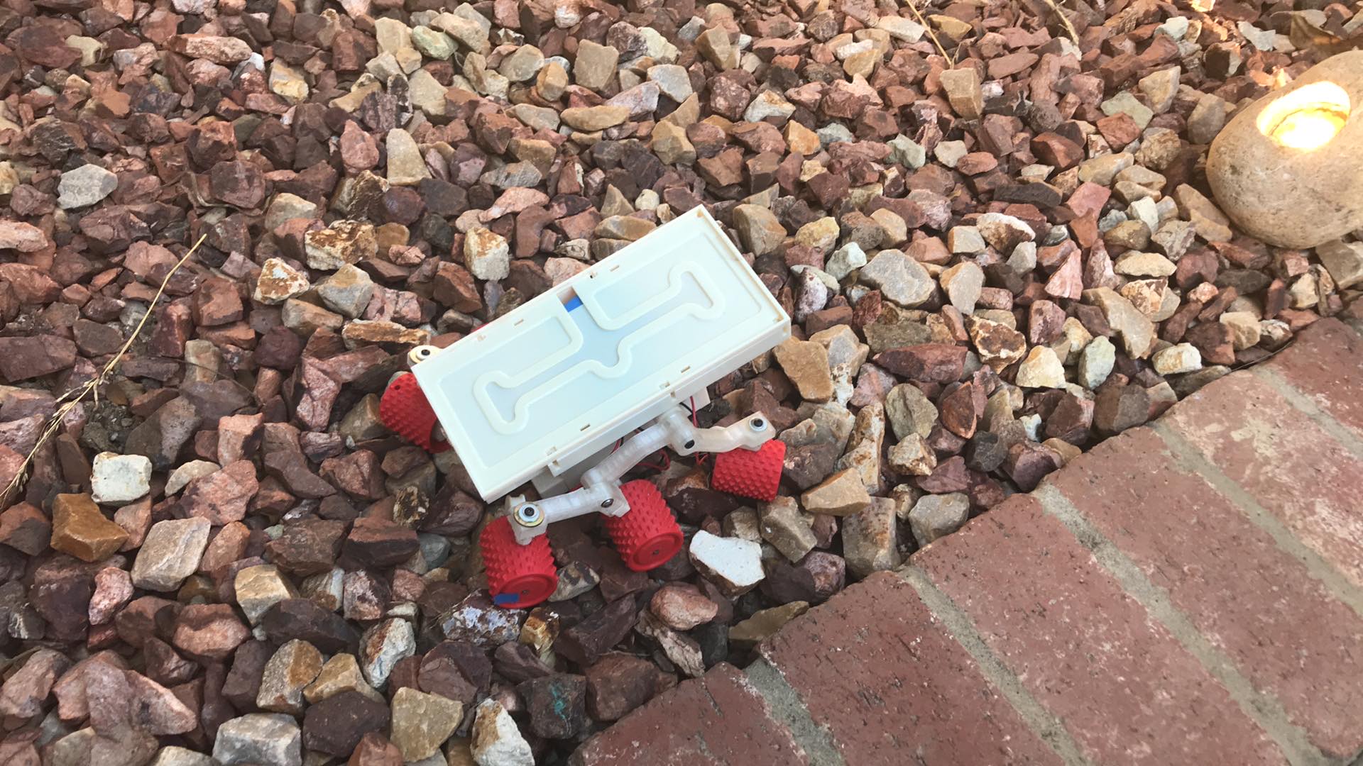
A track selected to approximate a martian terrain will be used to test the capabilities of the Sojourner robot.
The course will be designed in Electronics & Control Engineer Alex Dalton’s yard. Sojourner’s path will be plotted along a loop containing rocks and pebbles similar to the rough martian surface. From a natural and uneasy terrain, Sojourner will demonstrate the sensorless rotary encoders working to adjust the speed of each individual motor and look damn fine while it does.
Dependent on the validation of Sojourner’s research, Sojourner’s motors will be tested individually to test the accuracy of their sensorless encoding methods. Sensorless Encoding for Back EMF and Commutator Noise methods with the Polulu Motors will be compared against the Hall Effect Sensors designed for the Polulu Motors.
Any rocks along the path simulate a high-side event (slip), in which Sojourner reacts by diverting the power and energy of the unloaded wheel(s). The track will include an incline and a decline.
The above Sojourner Mission will be verified in early May on the test track and will be recorded and put into a demonstration video.
[/av_textblock]
[av_heading tag=’h2′ padding=’10’ heading=’Project Features’ color=” style=” custom_font=” size=” subheading_active=” subheading_size=’15’ custom_class=” admin_preview_bg=” av-desktop-hide=” av-medium-hide=” av-small-hide=” av-mini-hide=” av-medium-font-size-title=” av-small-font-size-title=” av-mini-font-size-title=” av-medium-font-size=” av-small-font-size=” av-mini-font-size=”][/av_heading]
[av_textblock size=” font_color=” color=” av-medium-font-size=” av-small-font-size=” av-mini-font-size=” admin_preview_bg=”]
Sojourner Body
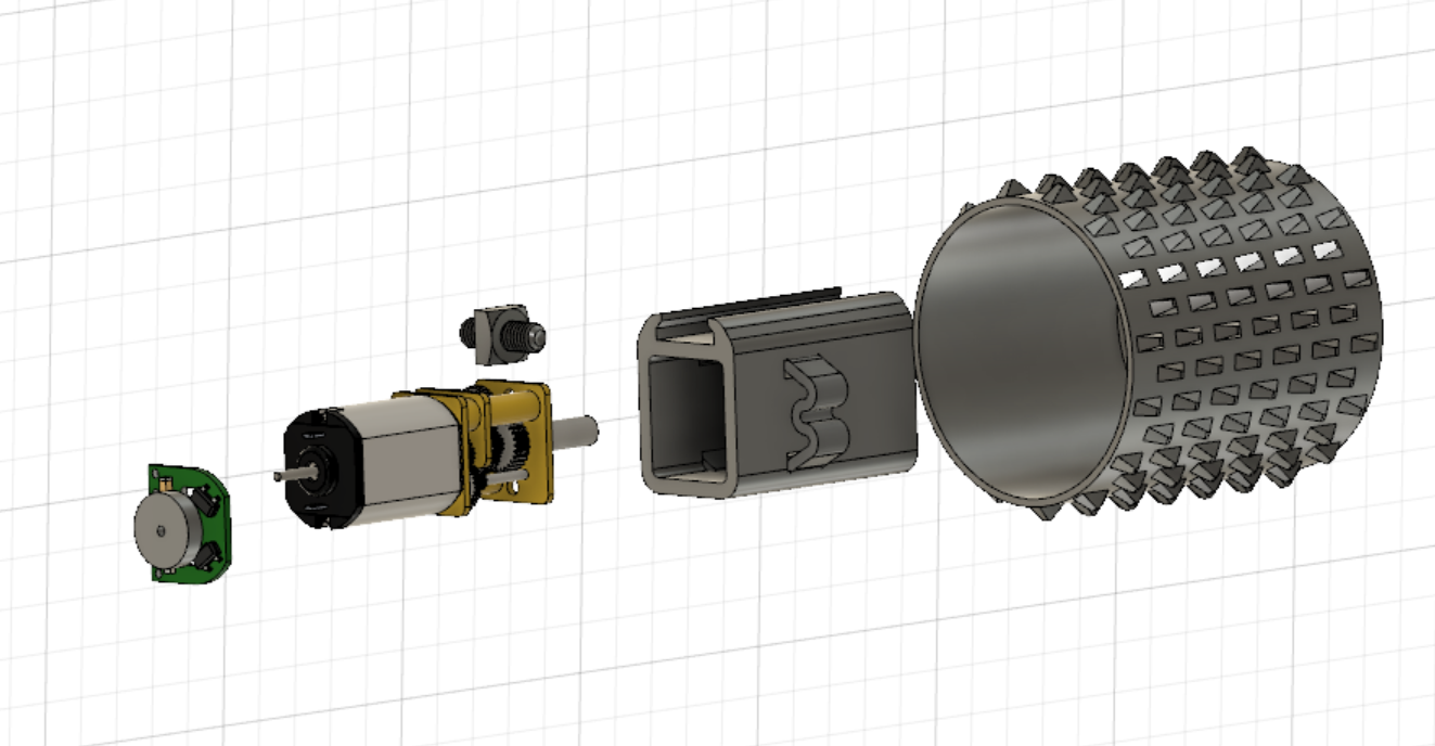
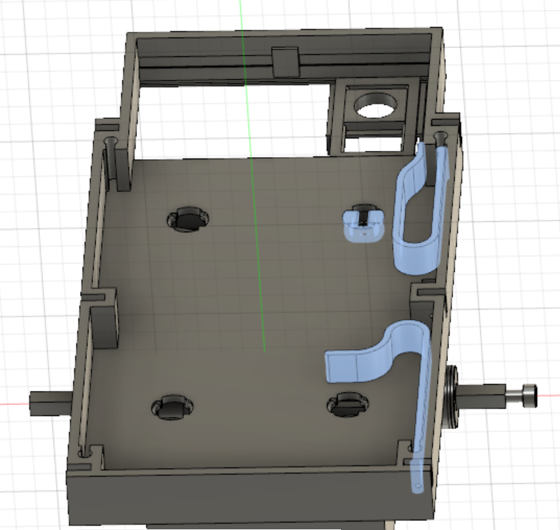
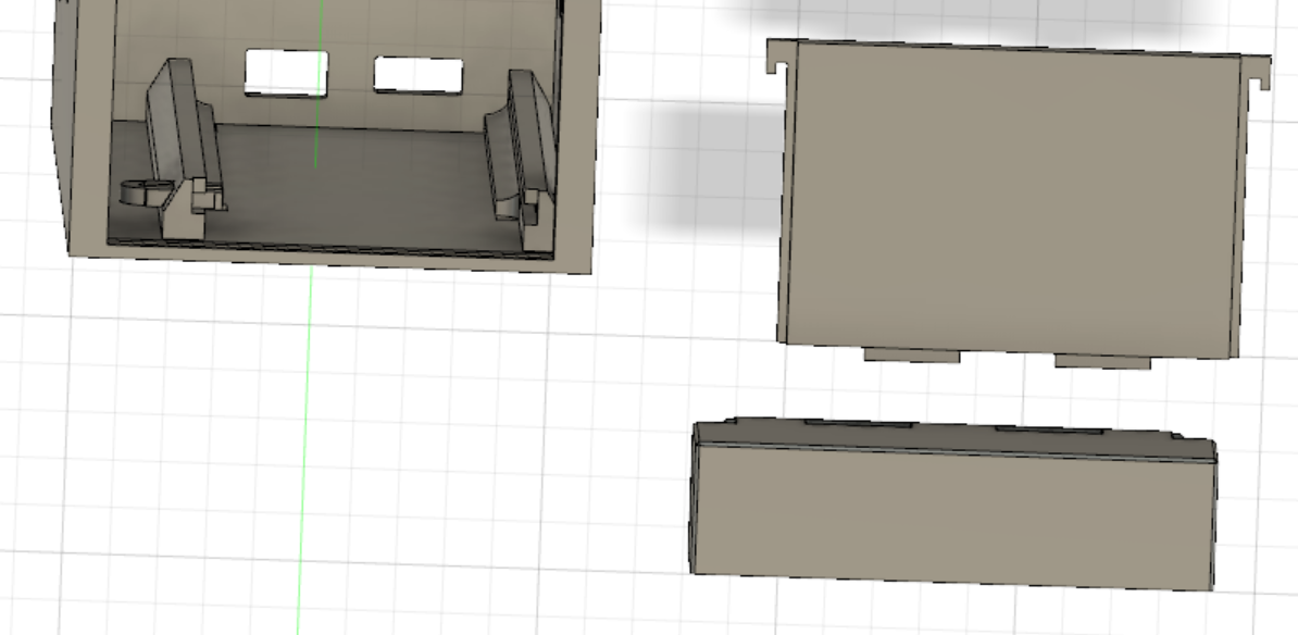
The four parts that split Sojourner into are the solar tray, phone holder, main chasis, and rocker bogie.
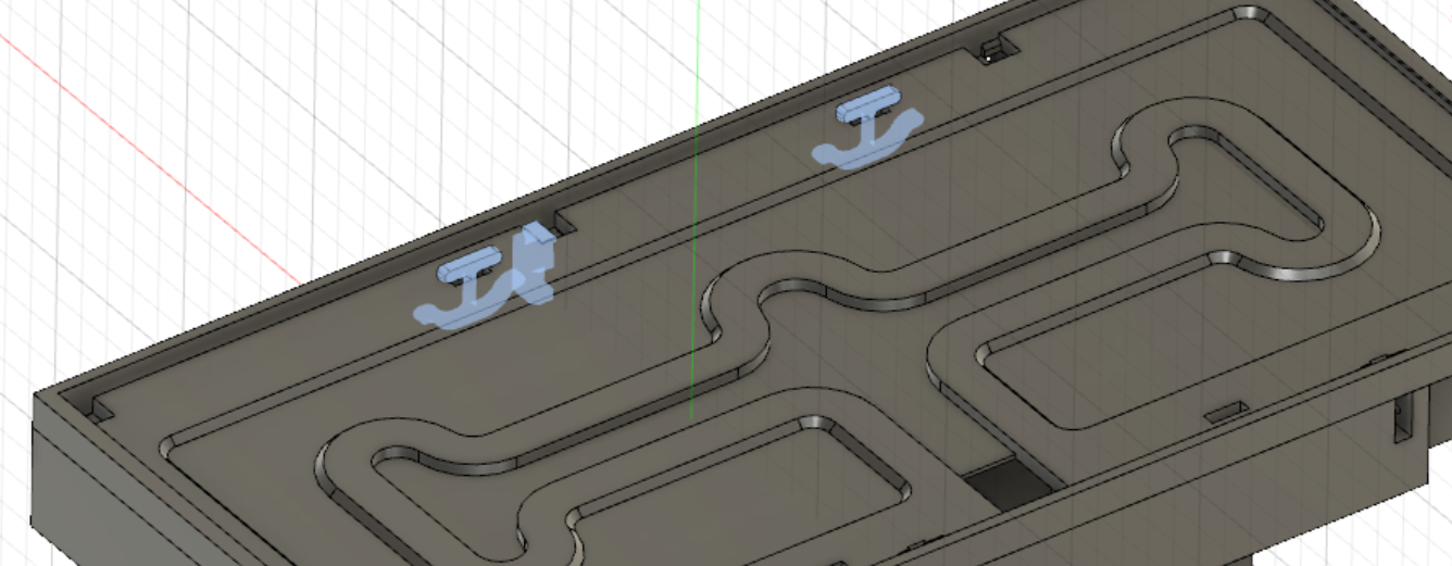
The solar tray holds the solar panels in the proper position to provide them with sunlight. This part also provides a cover for the phone holder. The phone holder has clips to keep the phone in the correct position to get video that can be displayed to the control panel. The main chasis holds the 3DoT microcontroller and has holes for the wires to connect to the wheels and servos.
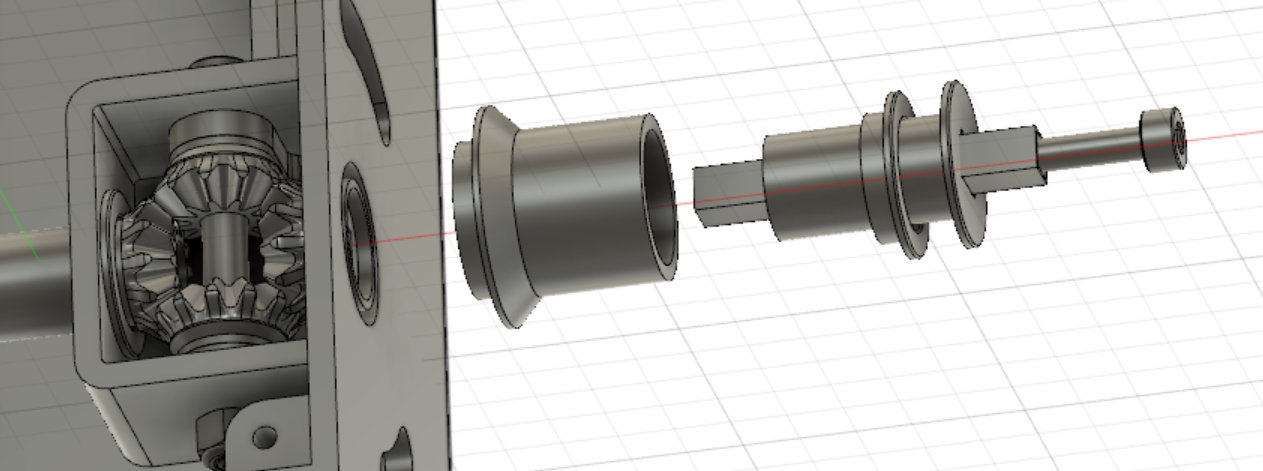
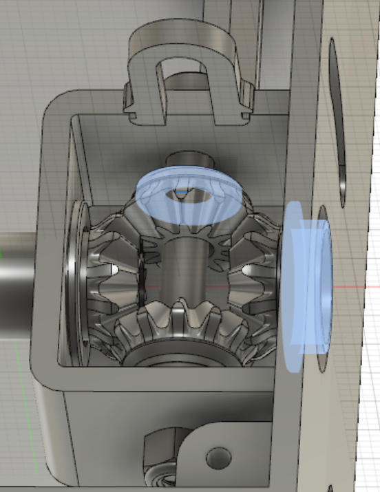
It holds the gearbox which keeps the two rocker bogies connected to the main chasis and moving in sync. The rocker bogie keeps are wheels in place and has mounts to connect the servos to the motors for steering. It is designed to help Sojourner overcome difficult terrain.
[/av_textblock]
[av_image src=’https://www.arxterra.com/wp-content/uploads/2020/05/Fusion1.png’ attachment=’162622′ attachment_size=’full’ align=’center’ styling=” hover=” link=” target=” caption=” font_size=” appearance=” overlay_opacity=’0.4′ overlay_color=’#000000′ overlay_text_color=’#ffffff’ animation=’no-animation’ admin_preview_bg=”][/av_image]
[av_textblock size=” font_color=” color=” av-medium-font-size=” av-small-font-size=” av-mini-font-size=” admin_preview_bg=”]
Figure 1- Sojourner Fusion Blowup View
[/av_textblock]
[av_textblock size=” font_color=” color=” av-medium-font-size=” av-small-font-size=” av-mini-font-size=” admin_preview_bg=”]
Sensorless Encoding
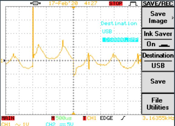
The commutator noise circuit starts with current sensing, which is then filtered by a band pass filter. There is a gain stage that also does some suppression of a large time constant introduced by the band pass filter. The use of a comparator configured for hysteresis is what allows for a clean transition at the spikes and avoids miscounting of peaks caused by standard noise in any system.
[/av_textblock]
[av_image src=’https://www.arxterra.com/wp-content/uploads/2020/05/comm-noise-labeled.jpg’ attachment=’162623′ attachment_size=’full’ align=’center’ styling=” hover=” link=” target=” caption=” font_size=” appearance=” overlay_opacity=’0.4′ overlay_color=’#000000′ overlay_text_color=’#ffffff’ animation=’no-animation’ admin_preview_bg=”][/av_image]
[av_textblock size=” font_color=” color=” av-medium-font-size=” av-small-font-size=” av-mini-font-size=” admin_preview_bg=”]
Figure 2- Commutator Noise Sensorless Encoding Circuit
[/av_textblock]
[av_heading tag=’h1′ padding=’10’ heading=’Requirements’ color=” style=’blockquote modern-quote’ custom_font=” size=” subheading_active=” subheading_size=’15’ custom_class=” admin_preview_bg=” av-desktop-hide=” av-medium-hide=” av-small-hide=” av-mini-hide=” av-medium-font-size-title=” av-small-font-size-title=” av-mini-font-size-title=” av-medium-font-size=” av-small-font-size=” av-mini-font-size=”][/av_heading]
[av_textblock size=” font_color=” color=” av-medium-font-size=” av-small-font-size=” av-mini-font-size=” admin_preview_bg=”]
Sojourner’s Requirements reflect the 5 main aspects of the project’s design. That being: the basic operations of Sojourner to match and iterate on prior generations, mission operation, the build of Sojourner, project logistics and research.
[/av_textblock]
[av_heading tag=’h2′ padding=’10’ heading=’Engineering Standards and Constraints ‘ color=” style=’blockquote modern-quote’ custom_font=” size=” subheading_active=” subheading_size=’15’ custom_class=” admin_preview_bg=” av-desktop-hide=” av-medium-hide=” av-small-hide=” av-mini-hide=” av-medium-font-size-title=” av-small-font-size-title=” av-mini-font-size-title=” av-medium-font-size=” av-small-font-size=” av-mini-font-size=”][/av_heading]
[av_textblock size=” font_color=” color=” av-medium-font-size=” av-small-font-size=” av-mini-font-size=” admin_preview_bg=”]
The Spring 2020 Sojourner team is aware of higher bodies of organization and the standards, codes and regulations they give when building a toy product. Below are those that apply to the Sojourner Project.
Applicable Engineering Standards
- Systems and Software Engineering — Life Cycle Processes –Requirements Engineering
- IEEE SCC21 – IEEE Approved Standard for Fuel Cells, Photovoltaics, Dispersed Generation, and Energy Storage
- NASA/SP-2007-6105 Rev1 – Systems Engineering Handbook
- Bluetooth Special Interest Group (SIG) Standard (supersedes IEEE 802.15.1)
- American Wire Gauge (AWG) Standard
- C++ standard (ISO/IEC 14882:1998)
- NXP Semiconductor, UM10204, I2C-bus specification and user manual.
- ATmega16U4/ATmega32U4, 8-bit Microcontroller with 16/32K bytes of ISP Flash and USB Controller datasheet section datasheet, Section 18, USART.
- USB 2.0 Specification released on April 27, 2000, usb_20_20180904.zip
- IEEE 29148-2018 – ISO/IEC/IEEE Approved Draft International Standard –
- Arduino De facto Standard scripting language and/or using the GCC C++ programming language, which is implements the ISO C++ standard (ISO/IEC 14882:1998) published in 1998, and the 2011 and 2014 revisions.
Environmental, Health, and Safety (EH&S) Standards
- CSULB COE Lab Safety
- CSULB Environmental Health & Safety
- IEEE National Electrical Safety Code
- NCEES Fundamental Handbook
- ASTM F963-17, compliant for Toy Safety
[/av_textblock]
[av_heading tag=’h2′ padding=’10’ heading=’Program Level 1 Requirements’ color=” style=’blockquote modern-quote’ custom_font=” size=” subheading_active=” subheading_size=’15’ custom_class=” admin_preview_bg=” av-desktop-hide=” av-medium-hide=” av-small-hide=” av-mini-hide=” av-medium-font-size-title=” av-small-font-size-title=” av-mini-font-size-title=” av-medium-font-size=” av-small-font-size=” av-mini-font-size=”][/av_heading]
[av_textblock size=” font_color=” color=” av-medium-font-size=” av-small-font-size=” av-mini-font-size=” admin_preview_bg=”]
Basic Operations
L1.1 Sojourner shall employ a custom PCB, to extend the capabilities of the 3DoT board to meet the Sojourner project and mission objectives including 4 DC motor drivers, and a method of sensorless encoding.
Criteria:
Aside from the 2 DC Motor and Servo Motor Spots on the 3DoT v9 shield, the Sojourner PCB shall add for the implementation of 4 extra DC Motors as well as 2 extra Servo Motors, as well as a method to take rpm data without the use of encoders.
L1.3 The ArxRobot App shall display the battery level of Sojourner.
Criteria:
The percentage of the battery level of Sojourner will be displayed on the ArxRobot App by selecting the widget.
Mission Operation
L1.5 Sojourner will be placed in a faux Mars Test Track.
Criteria:
Sojourner’s track to be tested on shall be composed of gravel, dirt and sand.
Sojourner Build
L1.4 Sojourner will be a scaled down version of the JPL mars rover in a scale of 4:1 for length, 7:2 for width, and 18:5 for height.
Criteria:
The Sojourner’s design is based on the JPL Mars Pathfinder. The dimensions of the pathfinder according to NASA JPL are: 65cm x 48 cm x 30 cm. Tolerance for this scale shall not exceed 10%.
L1.10 Sojourner will be designed so no wires are exposed.
Criteria:
Wires for the motors are fed through the holes in the PCB Compartment and are securely strapped onto the rocker bogie suspension using Zip Ties and electrical tape.
L1.11 The Sojourner will have any parts securely placed when given to the customer.
Criteria: All parts are screwed in and bolted down properly. No part will dismantle under a slight pull, when handed to the customer for submission.
L1.12 Assembly and reassembly in order to access the PCB of Sojourner will not take longer than 5 minutes, respectively.
Criteria:
Sojourners Solar Tray and Phone Cradle shall be able to be removed within 5 minutes to access the pcb) from a top-down perspective.
L1.17 Sojourner’s chassis will be 3D printed.
Criteria:
A 3D printed chassis, rocker bogie, phone cradle and phone tray, with material being PETG.
Project Logistics
L1.14 This Sojourner project shall not exceed $600.
Criteria:
To complete a functional Sojourner the cost shall not exceed $600.
L1.15
Sojourner will be compliant with applicable engineering standards, codes and regulations for software and documentation.
Criteria:
Sojourner code will be written in C++ in the Arduino app in order to meet the de facto C standard, while documentation meets the NASA Handbook.
L1.16 Sojourner will be compliant regarding environmental health and safety standards.
Criteria:
Sojourner will be compliant with also meet IEEE SCC21 proper fuel Storage methods and CSULB COE Lab Safety/Environmental Health and Safety. When not in use Sojourner’s battery shall be stored in a plastic bag, goggles will be worn while soldering.
Research
L1.22 Commutator Noise Sensorless Encoding shall be designed for a custom PCB.
Criteria:
PCB design is completed in EAGLE CAD, Cost should be minimized to under $30, assembled before May 12, 2020.
L1.25 Updated Motor Driver PCB shall add 5% more wire clearance on the edge.
Criteria:
Reduction of the size of the pcb on the side near the access of the on board DC Motors of the 3DoT should be reduced by at least 1 mm.
[/av_textblock]
[av_heading tag=’h2′ padding=’10’ heading=’Project Level 1 Functional Requirements’ color=” style=’blockquote modern-quote’ custom_font=” size=” subheading_active=” subheading_size=’15’ custom_class=” admin_preview_bg=” av-desktop-hide=” av-medium-hide=” av-small-hide=” av-mini-hide=” av-medium-font-size-title=” av-small-font-size-title=” av-mini-font-size-title=” av-medium-font-size=” av-small-font-size=” av-mini-font-size=”][/av_heading]
[av_textblock size=” font_color=” color=” av-medium-font-size=” av-small-font-size=” av-mini-font-size=” admin_preview_bg=”]
Basic Operations
L1.2 Sojourner’s DC Motors shall be able to be controlled by the ArxRobot App.
Criteria:
Through use of the Sliders on the Arxterra app, Sojourner’s DC motors will be able to turn 180 degrees forward and 180 degrees backward.
L1.26 Servo motors shall be able to turn 90 degrees.
Criteria:
User is to use the sliders on the ArxRobot App to turn a Servo Motor from rest to a 90-degree position.
Mission Operation
L1.6 Sojourner shall travel for 3 minutes
Criteria:
Sojourner shall not dismantle or pause for longer than 15 seconds within this time frame.
L1.7 Sojourner shall travel 10 feet.
Criteria:
10 Feet of consecutive motion.
L1.8 Sojourner shall travel an incline of 20 degrees.
Criteria:
Sojourner shall be able to travel up and down and incline of 20 degrees, this will be simulated on a ramp.
L1.9 Sojourner shall traverse a high side event.
Criteria:
Sojourner will divert power from rocker bogie in air to side with contact with the ground using Sensorless encoders without overturning the robot.
Research
L1.18 Back EMF measurements shall estimate RPM +- 15% compared to external tachometer.
Criteria:
The measurements shall be taken as the motor runs in forward position; the Back EMF measurements use the L298 Motor Driver to accept ADC Values.
L1.19 Commutator noise circuit shall translate commutator spikes into a square wave with a unique frequency as a function of RPM.
Criteria:
If frequency changes relative to rpm, the square wave should be able to be scaled in relation to this.
L1.20 Circular buffer code shall enable shaft encoder values to match external tachometer +-5%.
Criteria:
Encoder values are comparable to +- 5% of the tachometer values.
L1.21 Commutator Noise Circuit shall operate with compatible 3DoT Voltage Levels.
Criteria:
Circuit shall work on 5 Volts with a single 3.3 bias in their components.
L1.23 Motor Driver and Back EMF implantation on the Sojourner shall allow for stackable commutator noise PCB.
Criteria:
JST Headers have been changed to standard headers.
L1.24 Implementation of the Back EMF PCB design shall allow for bi-directional testing.
Criteria:
The design involves using 3 OPA 350 Operational Amplifiers, in the back EMF. This should theoretically let the ADC takes values of forward/backwards.
L1.27 Motor Driver Shield shall implement a method to minimize pins needed on 3DoT.
Criteria: Multiplexer uses 1 ADC pin to get reading from 4 motors, PWM Driver pin controls Multiplexer.
L1.28 The compatibility of sensorless encoding methods will be analyzed regarding motor driver diodes.
Criteria: Back EMF circuit is compatible with fly back diodes.
[/av_textblock]
[av_heading tag=’h2′ padding=’10’ heading=’System/Subsystem/Specifications Level 2 Requirements’ color=” style=’blockquote modern-quote’ custom_font=” size=” subheading_active=” subheading_size=’15’ custom_class=” admin_preview_bg=” av-desktop-hide=” av-medium-hide=” av-small-hide=” av-mini-hide=” av-medium-font-size-title=” av-small-font-size-title=” av-mini-font-size-title=” av-medium-font-size=” av-small-font-size=” av-mini-font-size=”][/av_heading]
[av_textblock size=” font_color=” color=” av-medium-font-size=” av-small-font-size=” av-mini-font-size=” admin_preview_bg=”]
The following Level 2 requirements are derived from the further needs of our level 1 requirements. As Level 1 requirements crossed into the territory of derived requirements, due to a changed Verification and Validation plan; Level 1 requirements covered a lot of what was intended for level 2.
[/av_textblock]
[av_textblock size=” font_color=” color=” av-medium-font-size=” av-small-font-size=” av-mini-font-size=” admin_preview_bg=”]
L2.1 Sojourner’s PCB will cost less then $10 (price per unit).
L2.2.1 The ArxRobot App will be able to interface with the Arxterra Control Panel.
L2.2.2 Sojourner’s motors will be able to be controlled by the Arxterra Control Panel.
L2.6 Sojourner will be able to be controlled by the user for 3 minutes
L2.8 Sojourner will be able to travel 8 feet up an incline of 20 degrees.
L2.10 Sojourner’s wires will be able to be fed and placed in the notches in the rocker bogie suspension.
L2.17.1 Sojourner’s 3D printed parts shall be durable and survive 3 mission tests.
L2.17.2 Sojourner’s 3D printed parts shall take no longer than 9 hours for a complete print.
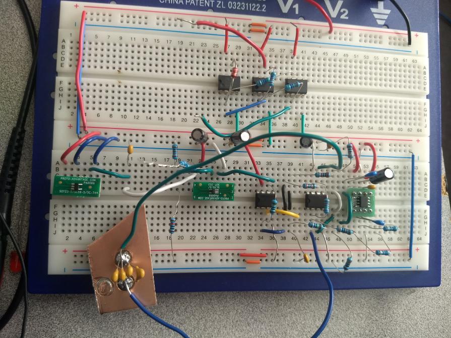
L2.22 Sojourner’s commutator noise circuit will be tested on a breadboard before PCB implementation.
[/av_textblock]
[av_heading tag=’h2′ padding=’10’ heading=’Allocated Requirements / System Resource Reports’ color=” style=’blockquote modern-quote’ custom_font=” size=” subheading_active=” subheading_size=’15’ custom_class=” admin_preview_bg=” av-desktop-hide=” av-medium-hide=” av-small-hide=” av-mini-hide=” av-medium-font-size-title=” av-small-font-size-title=” av-mini-font-size-title=” av-medium-font-size=” av-small-font-size=” av-mini-font-size=”][/av_heading]
[av_heading tag=’h3′ padding=’10’ heading=’Mass Shared Resource Report / Allocation’ color=” style=’blockquote modern-quote’ custom_font=” size=” subheading_active=” subheading_size=’15’ custom_class=” admin_preview_bg=” av-desktop-hide=” av-medium-hide=” av-small-hide=” av-mini-hide=” av-medium-font-size-title=” av-small-font-size-title=” av-mini-font-size-title=” av-medium-font-size=” av-small-font-size=” av-mini-font-size=”][/av_heading]
[av_image src=’https://www.arxterra.com/wp-content/uploads/2020/05/mass-report.jpg’ attachment=’162625′ attachment_size=’full’ align=’center’ styling=” hover=” link=” target=” caption=” font_size=” appearance=” overlay_opacity=’0.4′ overlay_color=’#000000′ overlay_text_color=’#ffffff’ animation=’no-animation’ admin_preview_bg=”][/av_image]
[av_textblock size=” font_color=” color=” av-medium-font-size=” av-small-font-size=” av-mini-font-size=” admin_preview_bg=”]
Figure 3 – Mass Report
[/av_textblock]
[av_textblock size=” font_color=” color=” av-medium-font-size=” av-small-font-size=” av-mini-font-size=” admin_preview_bg=”]
The estimated weight of our sojourned was repeated from previous versions as we were only printing the files that we were given without any change in the design. We measured each part after getting them from the printers as well as measured the loose nuts and bolts as a lump sum as. Our robot was very close to what we expected which confirmed our design fell well within spec and no obvious mistakes were made in the transition from one generation to another.
[/av_textblock]
[av_heading tag=’h3′ padding=’10’ heading=’Power Shared Resource Report / Allocation’ color=” style=’blockquote modern-quote’ custom_font=” size=” subheading_active=” subheading_size=’15’ custom_class=” admin_preview_bg=” av-desktop-hide=” av-medium-hide=” av-small-hide=” av-mini-hide=” av-medium-font-size-title=” av-small-font-size-title=” av-mini-font-size-title=” av-medium-font-size=” av-small-font-size=” av-mini-font-size=”][/av_heading]
[av_textblock size=” font_color=” color=” av-medium-font-size=” av-small-font-size=” av-mini-font-size=” admin_preview_bg=”]
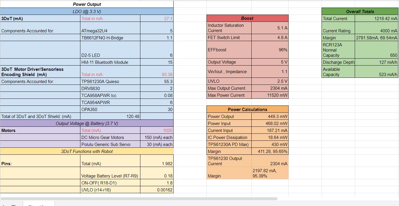
Figure 4 –Power Report
The equation for setting the current limiter of the 3DoT is 23950/(100*(N/128))^0.977mA, where N is the number of steps written to MCP4017 between 0 and 128. Our current N value is 64, which gives us a current limiter value of 524.1 mA. To increase the amount of current we can provide to our motors and servos we would want to lower this N value, but setting this value too low could cause the amount of current to damage the board.
When working with our robot, we noticed that the servos seem to be taking the most current when trying to move the gears connect to Sojourner’s wheels. Having this heavier load causes them to draw current past the current limiter. The same is also true for the motors in extreme circumstances, going from max speed in one direction to max speed in the opposite direction caused the current to reach its limit.
[/av_textblock]
[av_heading tag=’h1′ padding=’10’ heading=’Project Report’ color=” style=’blockquote modern-quote’ custom_font=” size=” subheading_active=” subheading_size=’15’ custom_class=” admin_preview_bg=” av-desktop-hide=” av-medium-hide=” av-small-hide=” av-mini-hide=” av-medium-font-size-title=” av-small-font-size-title=” av-mini-font-size-title=” av-medium-font-size=” av-small-font-size=” av-mini-font-size=”][/av_heading]
[av_textblock size=” font_color=” color=” av-medium-font-size=” av-small-font-size=” av-mini-font-size=” admin_preview_bg=”]
The PBS and WBS are shown below. Considering how the engineering method and structure for the work is set up, ours are quite different.
[/av_textblock]
[av_heading tag=’h2′ padding=’10’ heading=’Project WBS and PBS’ color=” style=’blockquote modern-quote’ custom_font=” size=” subheading_active=” subheading_size=’15’ custom_class=” admin_preview_bg=” av-desktop-hide=” av-medium-hide=” av-small-hide=” av-mini-hide=” av-medium-font-size-title=” av-small-font-size-title=” av-mini-font-size-title=” av-medium-font-size=” av-small-font-size=” av-mini-font-size=”][/av_heading]
[av_textblock size=” font_color=” color=” av-medium-font-size=” av-small-font-size=” av-mini-font-size=” admin_preview_bg=”]
The following diagram below shows our Project Work Breakdown Structure (WBS).
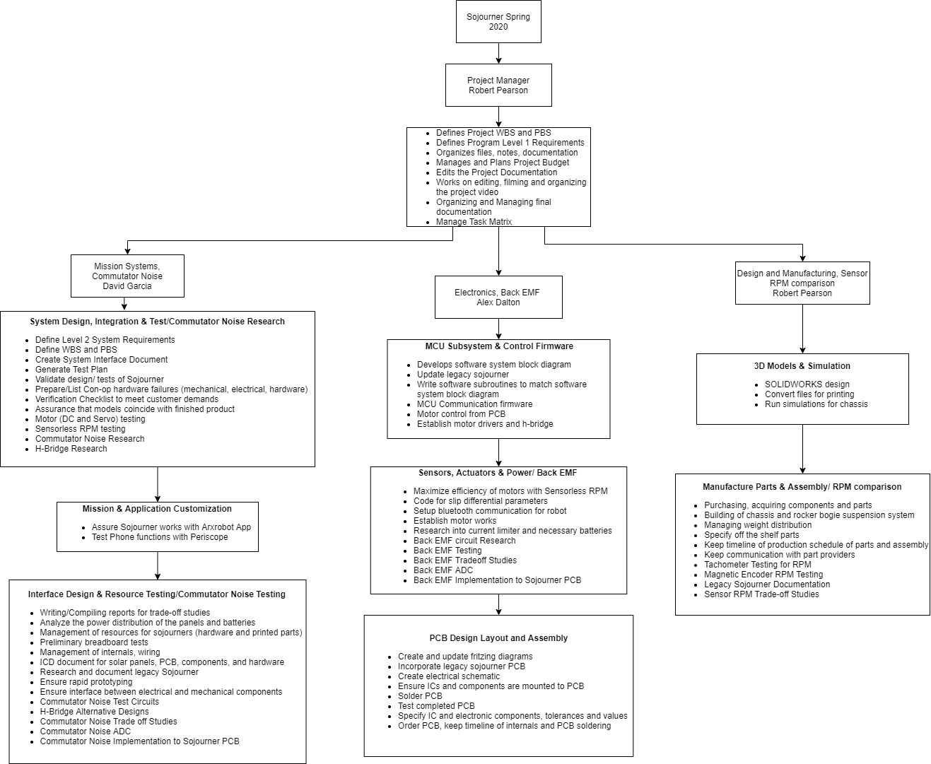
Figure 5 – WBS
The following diagram below shows our Project Breakdown Structure (PBS).

Figure 6 – PBS
[/av_textblock]
[av_textblock size=” font_color=” color=” av-medium-font-size=” av-small-font-size=” av-mini-font-size=” admin_preview_bg=”]
Considering our project focused heavily on research, the normal structure of the WBS and PBS would not suffice. In order to solve this problem, we initially split off the work load to fit into methods of encoding. Alex would research and start to implement the Back EMF method, while also focusing on Telemetry. Robert would analyze the Polulu Encoders while working on the management of the project, while David would set up the mission while working on Commutator Noise.
The PBS also better suited our need as it became clear which specific task of the project would be applied to whom. There was crossover between Alex’s code and David’s implementation of the circuits. As David had the oscilloscope and power supply it fell on him to test and have the circuits built.
[/av_textblock]
[av_heading tag=’h2′ padding=’10’ heading=’Cost’ color=” style=’blockquote modern-quote’ custom_font=” size=” subheading_active=” subheading_size=’15’ custom_class=” admin_preview_bg=” av-desktop-hide=” av-medium-hide=” av-small-hide=” av-mini-hide=” av-medium-font-size-title=” av-small-font-size-title=” av-mini-font-size-title=” av-medium-font-size=” av-small-font-size=” av-mini-font-size=”][/av_heading]
[av_textblock size=” font_color=” color=” av-medium-font-size=” av-small-font-size=” av-mini-font-size=” admin_preview_bg=”]
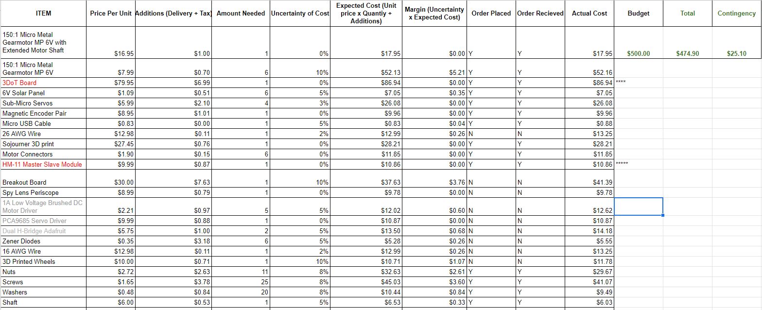
Figure 7 – Budget Spreadsheet
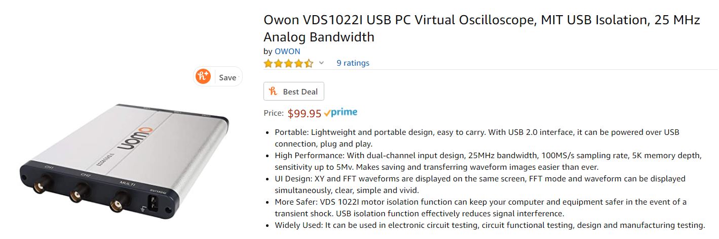
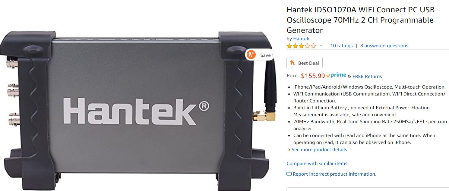
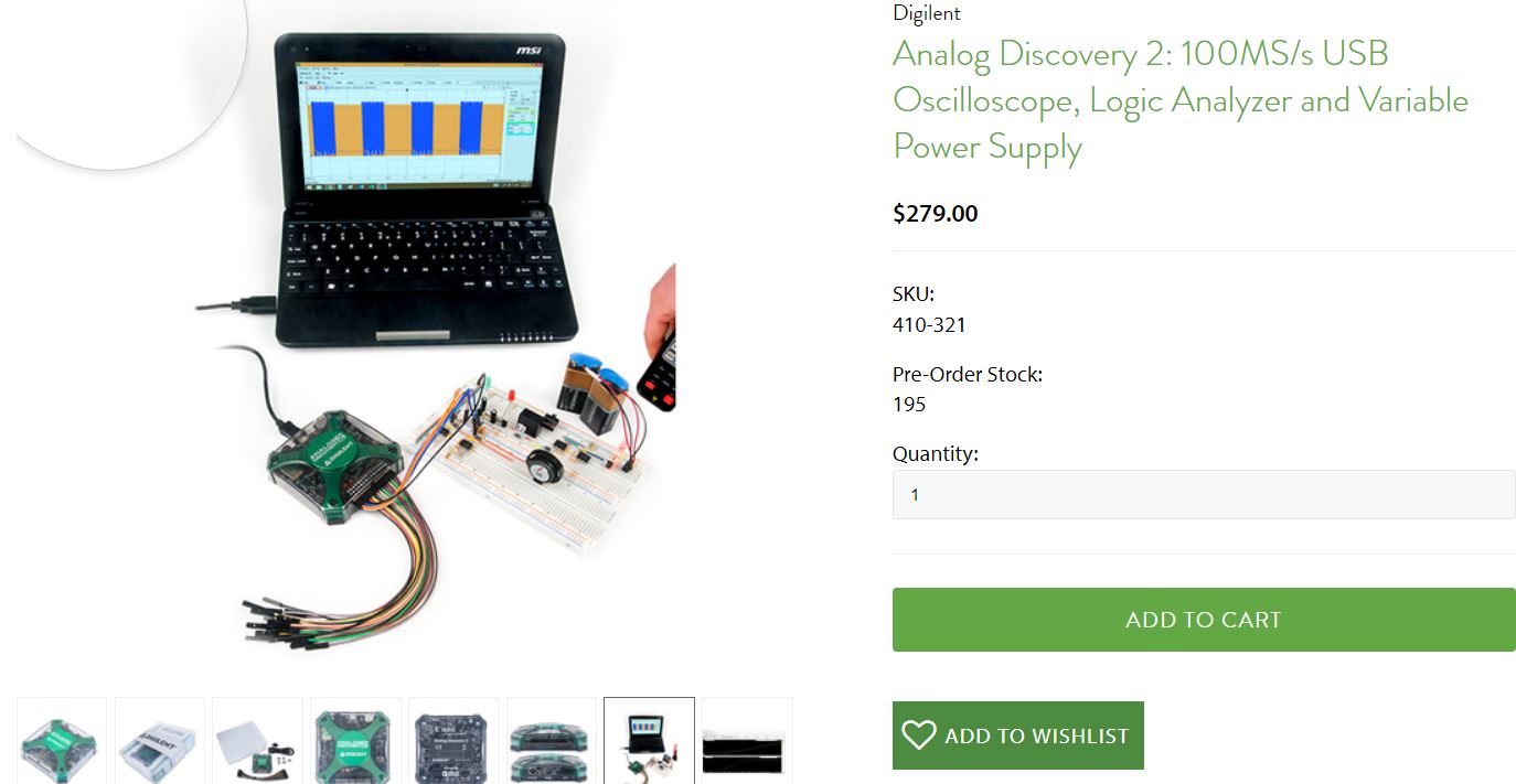
Sojourner’s cost reached a total of $577.56 with a contingency of $22.44 for a total of $600. One of the extra costs that came up later in the semester was buying a USB oscilloscope for David to continue testing. The total before the USB oscilloscope was $474.90 with a contingency of $125.10. For our project we had two members who are members of the Embedded Application Technology club and we would like to give a special thank you to them for funding our project.
[/av_textblock]
[av_heading tag=’h2′ padding=’10’ heading=’Schedule’ color=” style=’blockquote modern-quote’ custom_font=” size=” subheading_active=” subheading_size=’15’ custom_class=” admin_preview_bg=” av-desktop-hide=” av-medium-hide=” av-small-hide=” av-mini-hide=” av-medium-font-size-title=” av-small-font-size-title=” av-mini-font-size-title=” av-medium-font-size=” av-small-font-size=” av-mini-font-size=”][/av_heading]
[av_image src=’https://www.arxterra.com/wp-content/uploads/2020/05/Final-Schedule-May-9.jpg’ attachment=’162584′ attachment_size=’full’ align=’center’ styling=” hover=’av-hover-grow’ link=” target=” caption=” font_size=” appearance=” overlay_opacity=’0.4′ overlay_color=’#000000′ overlay_text_color=’#ffffff’ animation=’no-animation’ admin_preview_bg=”][/av_image]
[av_textblock size=” font_color=” color=” av-medium-font-size=” av-small-font-size=” av-mini-font-size=” admin_preview_bg=”]
Figure 8 – Schedule
[/av_textblock]
[av_textblock size=” font_color=” color=” av-medium-font-size=” av-small-font-size=” av-mini-font-size=” admin_preview_bg=”]
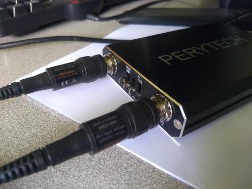
For this project, we had 3 critical paths for our project. These paths considered: Back EMF Sensorless Encoding, Commutator Noise Sensorless Encoding and the Main Sojourner Build/Code. These 3 tasks were designed around the idea of the 3 team members who were to work on these, David for Commutator Noise, Robert for Main Sojourner Build and Alex for Back EMF. Although as our project went into March the Stay At Home order was put into place. This order forced us to redesign the schedule for the project. Unfortunately, the schedule would face alot of tasks being pushed back. For example, since our team could not access oscilloscopes owned by the University, our team had to research and order one of our own. This pushed our testing back weeks. If parts broke during testing, shipping times also caused delays. We ran into this problem during the last weeks due to these unexpected delays, and were not able to fully complete the trade-off study as we had expected to. Our team had to base the trade-off study more so on cost and analog values than digital values.
[/av_textblock]
[av_heading tag=’h2′ padding=’10’ heading=’Burndown and/or Percent Complete’ color=” style=’blockquote modern-quote’ custom_font=” size=” subheading_active=” subheading_size=’15’ custom_class=” admin_preview_bg=” av-desktop-hide=” av-medium-hide=” av-small-hide=” av-mini-hide=” av-medium-font-size-title=” av-small-font-size-title=” av-mini-font-size-title=” av-medium-font-size=” av-small-font-size=” av-mini-font-size=”][/av_heading]
[av_image src=’https://www.arxterra.com/wp-content/uploads/2020/05/burndown.jpg’ attachment=’162585′ attachment_size=’full’ align=’center’ styling=” hover=’av-hover-grow’ link=” target=” caption=” font_size=” appearance=” overlay_opacity=’0.4′ overlay_color=’#000000′ overlay_text_color=’#ffffff’ animation=’no-animation’ admin_preview_bg=”][/av_image]
[av_textblock size=” font_color=” color=” av-medium-font-size=” av-small-font-size=” av-mini-font-size=” admin_preview_bg=”]
Figure 9 – Burndown Chart
[/av_textblock]
[av_textblock size=” font_color=” color=” av-medium-font-size=” av-small-font-size=” av-mini-font-size=” admin_preview_bg=”]
The burndown schedule displays the gaps in April in which we had to wait on receiving parts in order to get our circuits tested. Without them testing was stalled in this period of time. Because of this the final tests and the trade off study for the sensorless encoding were not formally completed.
[/av_textblock]
[av_heading tag=’h1′ padding=’10’ heading=’Concept and Preliminary Design’ color=” style=’blockquote modern-quote’ custom_font=” size=” subheading_active=” subheading_size=’15’ custom_class=” admin_preview_bg=” av-desktop-hide=” av-medium-hide=” av-small-hide=” av-mini-hide=” av-medium-font-size-title=” av-small-font-size-title=” av-mini-font-size-title=” av-medium-font-size=” av-small-font-size=” av-mini-font-size=”][/av_heading]
[av_textblock size=” font_color=” color=” av-medium-font-size=” av-small-font-size=” av-mini-font-size=” admin_preview_bg=”]
To adapt sensorless encoding to Sojourner, multiple iterations of the commutator noise and back EMF circuits had to be built. When testing these circuits, we would take note of the hardware complexity of the circuit, for the cost of implementation. We would also take a look at the accuracy and difficulty to implement the software to use the ADC properly
Commutator Noise
Unlike the method for back EMF sensing, commutator spikes need no special timing to monitor whether the motor is being supplied power or not. As long as the motor is spinning there will be commutator spikes inherent in the design and physical construction of the brushed DC motor. The challenge for this method was to get a way to reliably catch the sparks, filter the peaks in such a way as to be able to relate the frequency of the peaks to a number for RPM. Due to limitation of pins being allocated to motor sensing then we will have to also implement a MUX that can be used to reduce 10 lines to only 3 lines needed for each method.
Back EMF Circuit
As we began this project an initial stumbling block was the misnomer of back EMF. Back EMF, properly described, is the voltage generated while the motor is being supplied with a voltage. What we were actually tempting to do was to operate our motor as a generator. This meant we have to achieve several steps before anything like success could be reached. First, we had to be able to sense when the motor was being supplied with a voltage and when the motor was spinning due to inertia. Once that trigger was in place, we must devise a delay scheme such that we can reliably avoid sampling the initial voltage spikes caused by the motor suddenly switching from motoring to generating mode. Then, the ADC had to be connected to our motor and a sample was to be buffered and averaged. This process can then be repeated through a MUX and used to poll each motor during operation.
[/av_textblock]
[av_heading tag=’h2′ padding=’10’ heading=’Literature Review’ color=” style=’blockquote modern-quote’ custom_font=” size=” subheading_active=” subheading_size=’15’ custom_class=” admin_preview_bg=” av-desktop-hide=” av-medium-hide=” av-small-hide=” av-mini-hide=” av-medium-font-size-title=” av-small-font-size-title=” av-mini-font-size-title=” av-medium-font-size=” av-small-font-size=” av-mini-font-size=”][/av_heading]
[av_textblock size=” font_color=” color=” av-medium-font-size=” av-small-font-size=” av-mini-font-size=” admin_preview_bg=”]
The two main areas for this project were coding the 3Dot to control the Sojourner robot and designing a circuit which could be used for reading RPM without the need of encoders. The Arxterra section on using the 3Dot provided a lot of information to get us started on the app and coding for the 3Dot. Having a detailed list of the registers on the controller was absolutely required when coding accurate delays and sampling functions. In addition, having a map of the pins of the 3dot informed much of what had to be done with the design of our PCB
When it came time to start dealing with the motor controls of the 3Dot some resources from Adafruit provided a lot of guidance. They even had some example code which acted as much to seed for what we were doing in this project. The library provided for the chip was also used extensively to control the speed and direction of our motor being used.
The two main documents guiding our research and work was the Texas Instruments Ripple Counter Design guide, The Precision MicroDrives article of back EMF measurements. The Texas Instruments design guide was the basis for the ripple counting breadboard circuit as well the pcb built for testing. The TI design guide provided equations and examples of what you would need to fully flesh out what would be needed to translate spikes to a countable frequency.
The precision microdrives article provided a lot of information for the process of how to calculate RPM from turning the motor off and on. In addition, the first circuit used for testing was provided by this site. Eventually we replaced much of the switching mechanism with a different board but much of the sensing section of our testing circuit was based on what we learned from working with their circuit.
3. Adafruit
[/av_textblock]
[av_heading tag=’h2′ padding=’10’ heading=’Design Innovation’ color=” style=’blockquote modern-quote’ custom_font=” size=” subheading_active=” subheading_size=’15’ custom_class=” admin_preview_bg=” av-desktop-hide=” av-medium-hide=” av-small-hide=” av-mini-hide=” av-medium-font-size-title=” av-small-font-size-title=” av-mini-font-size-title=” av-medium-font-size=” av-small-font-size=” av-mini-font-size=”][/av_heading]
[av_textblock size=” font_color=” color=” av-medium-font-size=” av-small-font-size=” av-mini-font-size=” admin_preview_bg=”]
- Pin Reduction Scheme – Implementation of a multiplexer capable of switching two lines at a time is the only way to make both BEMF and Commutator noise measurements possible. By using a Texas Instruments CD4052 analog multiplexer, we can minimize the lines needed to be run from the motors to the sensors by placing the MUX physically close to the motor lines and only running four lines when previously we would need 2 lines per motor and an entire circuit needed from each line. This way minimizes costs and complexity.
- MUX configured PCD – This board implemented an active full bridge rectifier circuit on the existing motor board as well as connecting the MUX from the motor lines to the controller. The motor pins were also moved to the outer perimeter of the board to enable stacking in the future.
[/av_textblock]
[av_heading tag=’h2′ padding=’10’ heading=’Conceptual Design / Proposed Solution’ color=” style=’blockquote modern-quote’ custom_font=” size=” subheading_active=” subheading_size=’15’ custom_class=” admin_preview_bg=” av-desktop-hide=” av-medium-hide=” av-small-hide=” av-mini-hide=” av-medium-font-size-title=” av-small-font-size-title=” av-mini-font-size-title=” av-medium-font-size=” av-small-font-size=” av-mini-font-size=”][/av_heading]
[av_textblock size=” font_color=” color=” av-medium-font-size=” av-small-font-size=” av-mini-font-size=” admin_preview_bg=”]
A large problem with the choice to implement both back EMF and commutator noise was the space needed on any shield would have to be integrated into the existing motor controller board. Doing so poses several design obstacles.
- More complicated routing in design
- Likely need to increase to more than a two layer board.
- Possible excess parts for anyone not using this method.
Rather than attempt to fit the footprint of both boards onto the same size it was proposed to use two multiplexers and route the signals for one of the methods to an add on board. This method would also mean we can minimize the pins needed by either method and take on a scheme for polling the motor for RPM data at a predefined interval. While this polling may also increase the lag in response to torque needed at each motor it should be a problem for a toy to likely encounter.
[/av_textblock]
[av_heading tag=’h1′ padding=’10’ heading=’System Design / Final Design and Results’ color=” style=” custom_font=” size=” subheading_active=” subheading_size=’15’ custom_class=” admin_preview_bg=” av-desktop-hide=” av-medium-hide=” av-small-hide=” av-mini-hide=” av-medium-font-size-title=” av-small-font-size-title=” av-mini-font-size-title=” av-medium-font-size=” av-small-font-size=” av-mini-font-size=”][/av_heading]
[av_textblock size=” font_color=” color=” av-medium-font-size=” av-small-font-size=” av-mini-font-size=” admin_preview_bg=”]
The system design here discusses the code, 3D design and experimental results of our circuits. In this portion of the project we have implemented a method of sensorless encoding into our PCB, that being Back EMF.
We have also expanded upon the interface Matrix in accordance to this implementation. The design of the PCB also furthers the possibility of sensorless encoding implementation as it is designed in order to accept a stacked commutator noise PCB onto it.
[/av_textblock]
[av_heading tag=’h2′ padding=’10’ heading=’System Block Diagram’ color=” style=” custom_font=” size=” subheading_active=” subheading_size=’15’ custom_class=” admin_preview_bg=” av-desktop-hide=” av-medium-hide=” av-small-hide=” av-mini-hide=” av-medium-font-size-title=” av-small-font-size-title=” av-mini-font-size-title=” av-medium-font-size=” av-small-font-size=” av-mini-font-size=”][/av_heading]
[av_horizontal_gallery ids=’162635,162637′ height=’25’ size=’large’ links=’active’ lightbox_text=” link_dest=” gap=’large’ active=’enlarge’ initial=” control_layout=’av-control-default’ id=”]
[av_textblock size=” font_color=” color=” av-medium-font-size=” av-small-font-size=” av-mini-font-size=” admin_preview_bg=”]
Figures 10 and 11 – System Block Diagrams
[/av_textblock]
[av_textblock size=” font_color=” color=” av-medium-font-size=” av-small-font-size=” av-mini-font-size=” admin_preview_bg=”]
Our system block diagram separates the UI and battery features as parts that interface with the Sojourner DC and Servo Motors. These motors are controlled by the app and are researched was focused on eventually being able to send RPM data back from the motors to the control panel/Arxrobot app. The solar panels were planned to charge our robot’s battery similar to solar panels on JPL’s pathfinder robot. The robot’s battery level is then sent to the Arxrobot app. Motor speed control is to be enacted through sensorless encoding and the Arxrobot app’s sliders are used to control the speed and direction of our motors as well as the position of the servos.
The servo controller specifically interfaces with the two servos located on the 3DoT microcontroller. Since our new servos on the shield are on the same side as these ones, we use the same command to move the new servos in sync with the ones already on the 3DoT. The same method is used to control the motors, the two motors already on the 3DoT are controlled with the sliders and the four motors on the shield follow the direction and speed of these motors with two shield motors corresponding to one 3DoT motor. These shield motors are controlled with a pwm driver on the motor driver shield.
For our back emf pcb we included a multiplexer to control the signals sent to the full wave rectifier. This multiplexer is controlled through the Adafruit PCA9685 PWM driver IC. The multiplexer connects to the ADC on the 3DoT allowing us to receive rpm readings. All of these commands and telemetry are made possible with the use of the HM-11 on the 3DoT board.
[/av_textblock]
[av_heading tag=’h2′ padding=’10’ heading=’Interface Definition’ color=” style=” custom_font=” size=” subheading_active=” subheading_size=’15’ custom_class=” admin_preview_bg=” av-desktop-hide=” av-medium-hide=” av-small-hide=” av-mini-hide=” av-medium-font-size-title=” av-small-font-size-title=” av-mini-font-size-title=” av-medium-font-size=” av-small-font-size=” av-mini-font-size=”][/av_heading]
[av_image src=’https://www.arxterra.com/wp-content/uploads/2020/05/interface-matrix.jpg’ attachment=’162654′ attachment_size=’full’ align=’center’ styling=” hover=” link=” target=” caption=” font_size=” appearance=” overlay_opacity=’0.4′ overlay_color=’#000000′ overlay_text_color=’#ffffff’ animation=’no-animation’ admin_preview_bg=”][/av_image]
[av_textblock size=” font_color=” color=” av-medium-font-size=” av-small-font-size=” av-mini-font-size=” admin_preview_bg=”]
Figure 12- Interface Matrix
[/av_textblock]
[av_textblock size=” font_color=” color=” av-medium-font-size=” av-small-font-size=” av-mini-font-size=” admin_preview_bg=”]
For our interface matrix we are using the two header sections on the top of the 3DoT. We do not include the front headers because they are not used in this project.
[/av_textblock]
[av_heading tag=’h1′ padding=’10’ heading=’Modeling/Experimental Results’ color=” style=” custom_font=” size=” subheading_active=” subheading_size=’15’ custom_class=” admin_preview_bg=” av-desktop-hide=” av-medium-hide=” av-small-hide=” av-mini-hide=” av-medium-font-size-title=” av-small-font-size-title=” av-mini-font-size-title=” av-medium-font-size=” av-small-font-size=” av-mini-font-size=”][/av_heading]
[av_textblock size=” font_color=” color=” av-medium-font-size=” av-small-font-size=” av-mini-font-size=” admin_preview_bg=”]
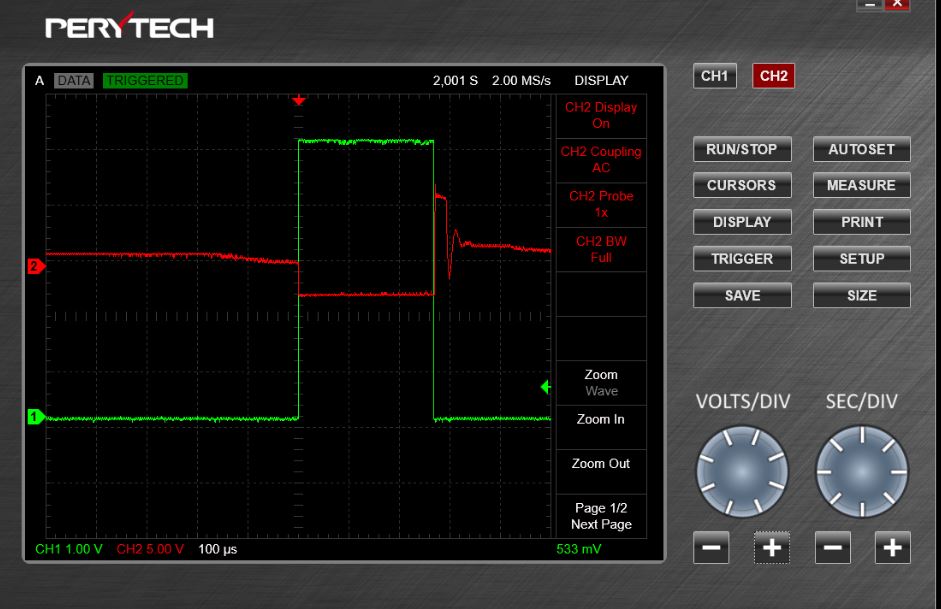
Much of the design process for the back EMF board was done simulating various configurations in LTSpice. Investigating the possibility of supplying a single supply to the op amps as opposed to a split supply. There was also investigation of some of the circuits found from the university of Northern Illinois.
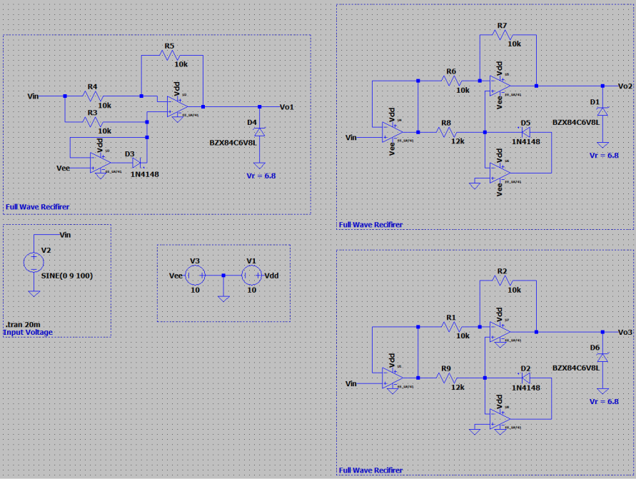
Figure 13 – LT SPICE EMF Circuit
One problem was the low supply available for the chips. In the simulation we would often see clipping to the supply rail.

Figure 14 – LT SPICE EMF Circuit Output
One of the configurations that seemed to work well was from the university of northern Illinois. We needed a supply of 8 volts but with the right gain we could be a very even graph.
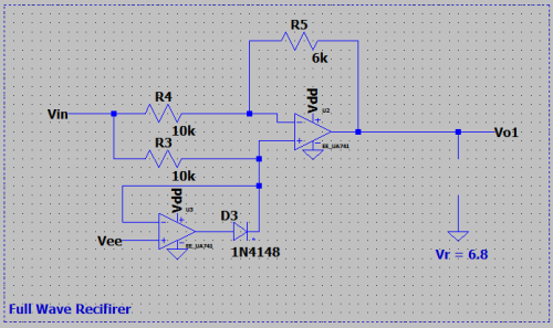
Figure 14 – Full wave Rectifier
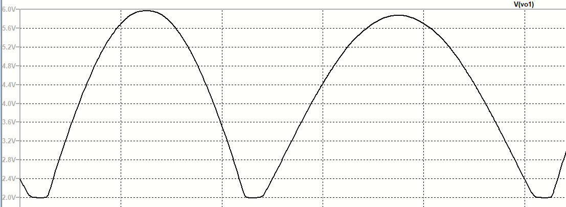
Figure 15 – Full wave Rectifier Output
We might consider feeding a full bridge rectified into a common emitter or common source configuration to give us a signal in the range of what we can achieve without a higher voltage.
[/av_textblock]
[av_heading tag=’h1′ padding=’10’ heading=’Mission Command and Control’ color=” style=” custom_font=” size=” subheading_active=” subheading_size=’15’ custom_class=” admin_preview_bg=” av-desktop-hide=” av-medium-hide=” av-small-hide=” av-mini-hide=” av-medium-font-size-title=” av-small-font-size-title=” av-mini-font-size-title=” av-medium-font-size=” av-small-font-size=” av-mini-font-size=”][/av_heading]
[av_image src=’https://www.arxterra.com/wp-content/uploads/2020/05/Arxrobot_App.png’ attachment=’162657′ attachment_size=’full’ align=’center’ styling=” hover=” link=” target=” caption=” font_size=” appearance=” overlay_opacity=’0.4′ overlay_color=’#000000′ overlay_text_color=’#ffffff’ animation=’no-animation’ admin_preview_bg=”][/av_image]
[av_textblock size=” font_color=” color=” av-medium-font-size=” av-small-font-size=” av-mini-font-size=” admin_preview_bg=”]
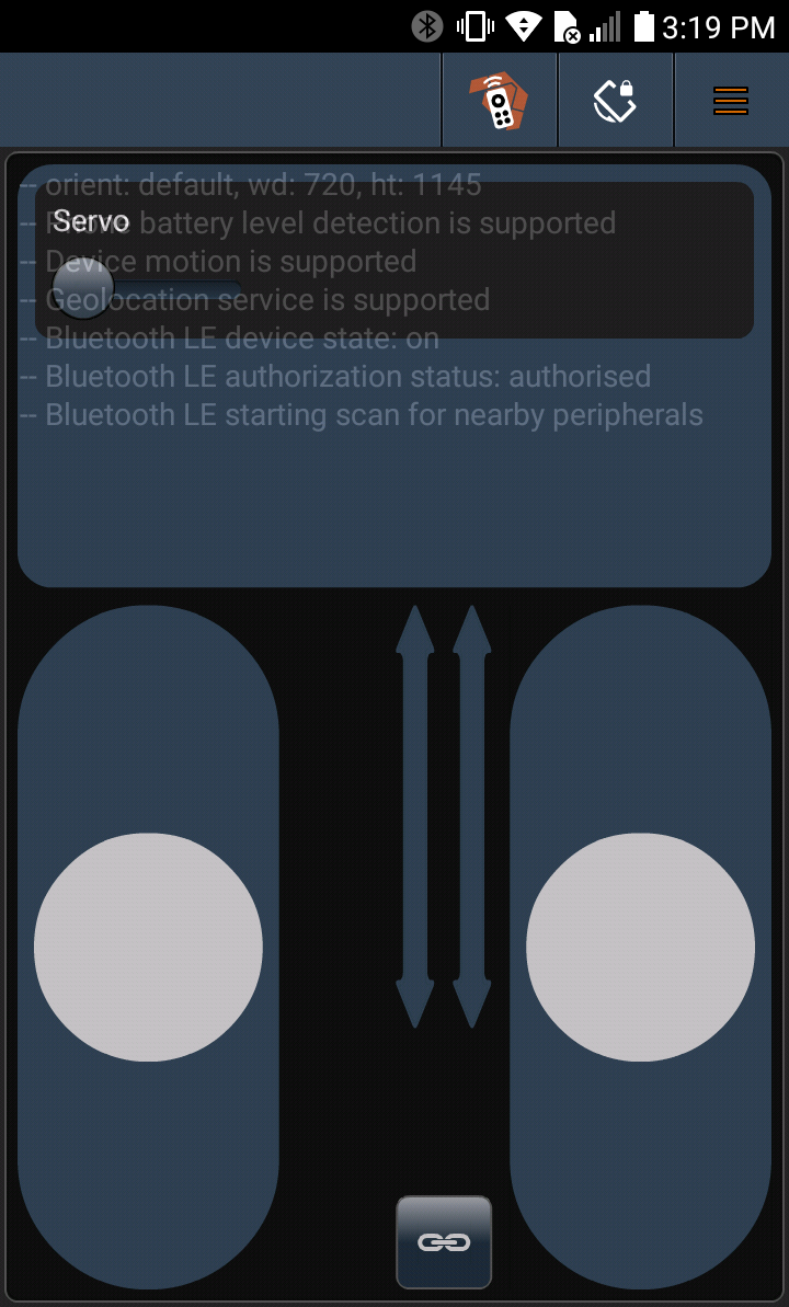
Figure 16 – Arxrobot App Controls
[/av_textblock]
[av_textblock size=” font_color=” color=” av-medium-font-size=” av-small-font-size=” av-mini-font-size=” admin_preview_bg=”]
#include
#include // instantiated as ArxRobot at end of class header
#include
#include // I2C support
//#define MCP4017_ADDRESS 0x2F
Adafruit_PWMServoDriver pwm = Adafruit_PWMServoDriver();
//servodriver is used for the 4 motors and 2 servos on the pcb shield
ArxRobot ArxRobot; // instantiated as ArxRobot at end of class header
Servo servoA; // Instantiate new Servo object
Servo servoB;
Servo servoC;
Servo servoD;
#define SERVO_C 22
#define SERVO_D 17
//these are the two new commands we are adding, move is an old command that we are changing
#define BLINK 0x40
#define SERVO 0x41
Motor motorA; //create motor A
Motor motorB; //create motor B
const uint8_t CMD_LIST_SIZE = 3; // we are adding 3 commands (MOVE, BLINK, SERVO)
/*
* User Defined Command BLINK (0x40) Example
* A5 01 40 E4
*/
void blinkHandler (uint8_t cmd, uint8_t param[], uint8_t n)
{
Serial1.write(cmd); // blink command = 0x40
Serial1.write(n); // number of param = 0
for (int i=0;i<n;i++) // param = none
{
// Serial.write (param[i]);
}
} // blinkHandler
/*
* Override MOVE (0x01) Command Example
* A5 05 01 01 80 01 80 A1
*/
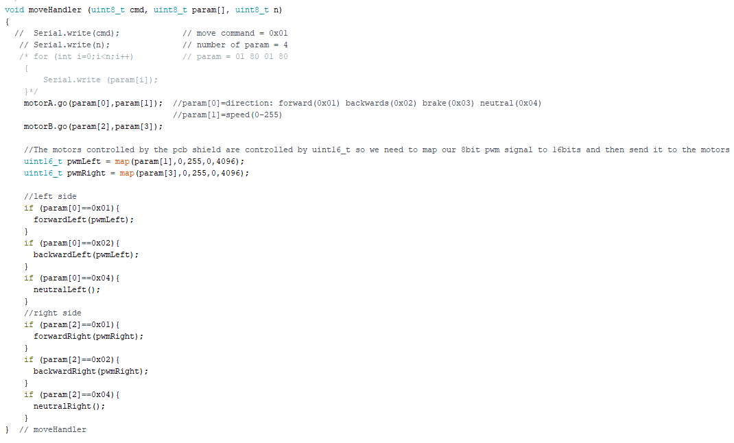
void moveHandler (uint8_t cmd, uint8_t param[], uint8_t n)
{
// Serial.write(cmd); // move command = 0x01
// Serial.write(n); // number of param = 4
/* for (int i=0;i<n;i++) // param = 01 80 01 80
{
Serial.write (param[i]);
}*/
motorA.go(param[0],param[1]); //param[0]=direction: forward(0x01) backwards(0x02) brake(0x03) neutral(0x04)
//param[1]=speed(0-255)
motorB.go(param[2],param[3]);
//The motors controlled by the pcb shield are controlled by uint16_t so we need to map our 8bit pwm signal to 16bits and then send it to the motors
uint16_t pwmLeft = map(param[1],0,255,0,4096);
uint16_t pwmRight = map(param[3],0,255,0,4096);
//left side
if (param[0]==0x01){
forwardLeft(pwmLeft);
}
if (param[0]==0x02){
backwardLeft(pwmLeft);
}
if (param[0]==0x04){
neutralLeft();
}
//right side
if (param[2]==0x01){
forwardRight(pwmRight);
}
if (param[2]==0x02){
backwardRight(pwmRight);
}
if (param[2]==0x04){
neutralRight();
}
} // moveHandler
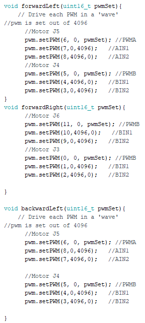
void forwardLeft(uint16_t pwmSet){
// Drive each PWM in a ‘wave’
//pwm is set out of 4096
//Motor J5
pwm.setPWM(6, 0, pwmSet); //PWMA
pwm.setPWM(7,0,4096); //AIN1
pwm.setPWM(8,4096,0); //AIN2
//Motor J4
pwm.setPWM(5, 0, pwmSet); //PWMB
pwm.setPWM(4,4096,0); //BIN1
pwm.setPWM(3,0,4096); //BIN2
}
void forwardRight(uint16_t pwmSet){
//Motor J6
pwm.setPWM(11, 0, pwmSet); //PWMB
pwm.setPWM(10,4096,0); //BIN1
pwm.setPWM(9,0,4096); //BIN2
//Motor J3
pwm.setPWM(0, 0, pwmSet); //PWMB
pwm.setPWM(1,0,4096); //BIN1
pwm.setPWM(2,4096,0); //BIN2
}
void backwardLeft(uint16_t pwmSet){
// Drive each PWM in a ‘wave’
//pwm is set out of 4096
//Motor J5
pwm.setPWM(6, 0, pwmSet); //PWMA
pwm.setPWM(8,0,4096); //AIN1
pwm.setPWM(7,4096,0); //AIN2
//Motor J4
pwm.setPWM(5, 0, pwmSet); //PWMB
pwm.setPWM(4,0,4096); //BIN1
pwm.setPWM(3,4096,0); //BIN2
}
void backwardRight(uint16_t pwmSet){
//Motor J6
pwm.setPWM(11, 0, pwmSet); //PWMB
pwm.setPWM(9,4096,0); //BIN1
pwm.setPWM(10,0,4096); //BIN2
//Motor J3
pwm.setPWM(0, 0, pwmSet); //PWMB
pwm.setPWM(1,4096,0); //BIN1
pwm.setPWM(2,0,4096); //BIN2
}
void neutralLeft(){
// Drive each PWM in a ‘wave’
//pwm is set out of 4096
//Motor J5
pwm.setPWM(7,0,4096); //AIN1
pwm.setPWM(8,0,4096); //AIN2
//Motor J4
pwm.setPWM(4,0,4096); //BIN1
pwm.setPWM(3,0,4096); //BIN2
}
void neutralRight(){
//Motor J3
pwm.setPWM(1,0,4096); //BIN1
pwm.setPWM(2,0,4096); //BIN2
//Motor J6
pwm.setPWM(9,0,4096); //BIN1
pwm.setPWM(10,0,4096); //BIN2
}
/*
* User Defined Command SERVO (0x41) Example
* Rotate servo to 90 degrees
* A5 02 41 90 76
*/
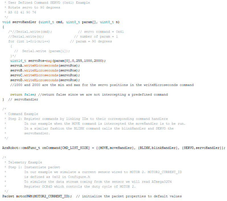
void servoHandler (uint8_t cmd, uint8_t param[], uint8_t n)
{
/*//Serial.write(cmd); // servo command = 0x41
//Serial.write(n); // number of param = 1
for (int i=0;i<n;i++) // param = 90 degrees
{
// Serial.write (param[i]);
}*/
uint16_t servoPos=map(param[0],0,255,1000,2000);
servoA.writeMicroseconds(servoPos);
servoB.writeMicroseconds(servoPos);
servoC.writeMicroseconds(servoPos);
servoD.writeMicroseconds(servoPos);
//1000 and 2000 are the min and max for the servo positions in the writeMicroseconds command
return false; //return false since we are not intercepting a predefined command
} // servoHandler
/*
* Command Example
* Step 2: Register commands by linking IDs to their corresponding command handlers
* In our example when the MOVE command is intercepted the moveHandler is to be run.
* In a similar fashion the BLINK command calls the blinkHandler and SERVO the
* servoHandler.
*/
ArxRobot::cmdFunc_t onCommand[CMD_LIST_SIZE] = {{MOVE,moveHandler}, {BLINK,blinkHandler}, {SERVO,servoHandler}};
/*
* Telemetry Example
* Step 1: Instantiate packet
* In our example we simulate a current sensor wired to MOTOR 2. MOTOR2_CURRENT_ID
* is defined as 0x02 in Configure.h
* To simulate the data stream coming from the sensor we will read ATmega32U4
* Register OCR4D which controls the duty cycle of MOTOR 2.
*/
Packet motorPWM(MOTOR2_CURRENT_ID); // initialize the packet properties to default values
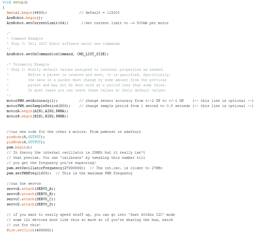
void setup()
{
Serial.begin(9600); // default = 115200
ArxRobot.begin();
ArxRobot.setCurrentLimit(64); //set current limit to ~= 500mA per motor
/*
* Command Example
* Step 3: Tell 3DoT Robot software about new commands
*/
ArxRobot.setOnCommand(onCommand, CMD_LIST_SIZE);
/* Telemetry Example
* Step 2: Modify default values assigned to internal properties as needed.
* Before a packet is created and sent, it is qualified. Specifically,
* the data in a packet must change by some amount from the previous
* packet and may not be sent with at a period less than some value.
* In most cases you can leave these values at their default values.
*/
motorPWM.setAccuracy(1); // change sensor accuracy from +/-2 DN to +/-1 DN (– this line is optional –)
motorPWM.setSamplePeriod(500); // change sample period from 1 second to 0.5 seconds (– this line is optional –)
motorA.begin(AIN1,AIN2,PWMA);
motorB.begin(BIN1,BIN2,PWMB);
//our new code for the other 4 motors. From pwmtest on adafruit
pinMode(5,OUTPUT);
pinMode(6,OUTPUT);
pwm.begin();
// In theory the internal oscillator is 25MHz but it really isn’t
// that precise. You can ‘calibrate’ by tweaking this number till
// you get the frequency you’re expecting!
pwm.setOscillatorFrequency(27000000); // The int.osc. is closer to 27MHz
pwm.setPWMFreq(1600); // This is the maximum PWM frequency
//run the servos
servoA.attach(SERVO_A);
servoB.attach(SERVO_B);
servoC.attach(SERVO_C);
servoD.attach(SERVO_D);
// if you want to really speed stuff up, you can go into ‘fast 400khz I2C’ mode
// some i2c devices dont like this so much so if you’re sharing the bus, watch
// out for this!
Wire.setClock(400000);
}
void loop()
{
ArxRobot.loop();
}
[/av_textblock]
[av_textblock size=” font_color=” color=” av-medium-font-size=” av-small-font-size=” av-mini-font-size=” admin_preview_bg=”]
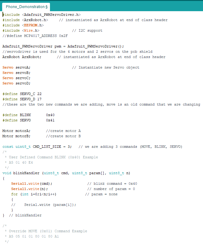
For our commands we use a modified move command and a custom servo command.
Move(0x01)- This command is prebuild into the the Arxrobot app. We are overriding this command by adding four more additional motors to be run. Each side has one motor directly connected to the 3DoT that receives commands telling it direction and speed as normal. The two additional motors on each side of the robot use the same command to determine direction and the speed value is converted to a value that is usable by the PCA9685PW to determine their speed. We use sliders for this command so we can change Sojourners speed and can unlink the two sliders to change direction.
Servo(0x41)- This command is an unisgned 8 bit integer that determines the postion of the four servos on Sojourner. Similar to move, two of our servos are connected directly to the 3DoT while the two other servos are connect to the motor driver shield. This new command determines the position of the servos between 0 and 90 degrees. We use a slider so we can position the servos anywhere between these two values.
[/av_textblock]
[av_heading tag=’h1′ padding=’10’ heading=’Electronic Design’ color=” style=” custom_font=” size=” subheading_active=” subheading_size=’15’ custom_class=” admin_preview_bg=” av-desktop-hide=” av-medium-hide=” av-small-hide=” av-mini-hide=” av-medium-font-size-title=” av-small-font-size-title=” av-mini-font-size-title=” av-medium-font-size=” av-small-font-size=” av-mini-font-size=”][/av_heading]
[av_textblock size=” font_color=” color=” av-medium-font-size=” av-small-font-size=” av-mini-font-size=” admin_preview_bg=”]
Out electronics Design consisted of working on two circuits, a Back EMF circuit and a Commutator noise circuit. The back EMF circuit was designed to be integrated on the existing 3 dot motor board while the commutator noise circuit was to be a board that could be turned into a stackable board for expansion in later generations.
[/av_textblock]
[av_heading tag=’h2′ padding=’10’ heading=’PCB Design’ color=” style=” custom_font=” size=” subheading_active=” subheading_size=’15’ custom_class=” admin_preview_bg=” av-desktop-hide=” av-medium-hide=” av-small-hide=” av-mini-hide=” av-medium-font-size-title=” av-small-font-size-title=” av-mini-font-size-title=” av-medium-font-size=” av-small-font-size=” av-mini-font-size=”][/av_heading]
[av_heading tag=’h3′ padding=’10’ heading=’Commutator Noise PCB’ color=” style=” custom_font=” size=” subheading_active=” subheading_size=’15’ custom_class=” admin_preview_bg=” av-desktop-hide=” av-medium-hide=” av-small-hide=” av-mini-hide=” av-medium-font-size-title=” av-small-font-size-title=” av-mini-font-size-title=” av-medium-font-size=” av-small-font-size=” av-mini-font-size=”][/av_heading]
[av_image src=’https://www.arxterra.com/wp-content/uploads/2020/05/Comm-noise-pcb.jpg’ attachment=’162648′ attachment_size=’full’ align=’center’ styling=” hover=” link=” target=” caption=” font_size=” appearance=” overlay_opacity=’0.4′ overlay_color=’#000000′ overlay_text_color=’#ffffff’ animation=’no-animation’ admin_preview_bg=”][/av_image]
[av_textblock size=” font_color=” color=” av-medium-font-size=” av-small-font-size=” av-mini-font-size=” admin_preview_bg=”]
Figure 17 – Commutator Noise PCB
[/av_textblock]
[av_textblock size=” font_color=” color=” av-medium-font-size=” av-small-font-size=” av-mini-font-size=” admin_preview_bg=”]
The final aim of this board was to be capable of being mounted onto 3Dot board as an expansion module. During the course of our work we realized trying to fit everything on one board would be impractical so there would have to be a second board that can deal with the commutator noise circuit and only pass back the square wave. The test board was designed to fit only a footprint similar to the 3 dot itself as to be easily adapted to an adapter board.
An advantage of building the circuit outlined in the TI design guide is that the voltages needed are the same as the native 3Dot voltages. Each chip runs on 5 volts with a single 3.3 volt bias needed at the output.
[/av_textblock]
[av_heading tag=’h3′ padding=’10’ heading=’Motor Driver/ Back EMF PCB’ color=” style=” custom_font=” size=” subheading_active=” subheading_size=’15’ custom_class=” admin_preview_bg=” av-desktop-hide=” av-medium-hide=” av-small-hide=” av-mini-hide=” av-medium-font-size-title=” av-small-font-size-title=” av-mini-font-size-title=” av-medium-font-size=” av-small-font-size=” av-mini-font-size=”][/av_heading]
[av_image src=’https://www.arxterra.com/wp-content/uploads/2020/05/PCB-design.jpg’ attachment=’162659′ attachment_size=’full’ align=’center’ styling=” hover=” link=” target=” caption=” font_size=” appearance=” overlay_opacity=’0.4′ overlay_color=’#000000′ overlay_text_color=’#ffffff’ animation=’no-animation’ admin_preview_bg=”][/av_image]
[av_textblock size=” font_color=” color=” av-medium-font-size=” av-small-font-size=” av-mini-font-size=” admin_preview_bg=”]
Figure 18 – Motor Driver/ Back EMF PCB
[/av_textblock]
[av_textblock size=” font_color=” color=” av-medium-font-size=” av-small-font-size=” av-mini-font-size=” admin_preview_bg=”]
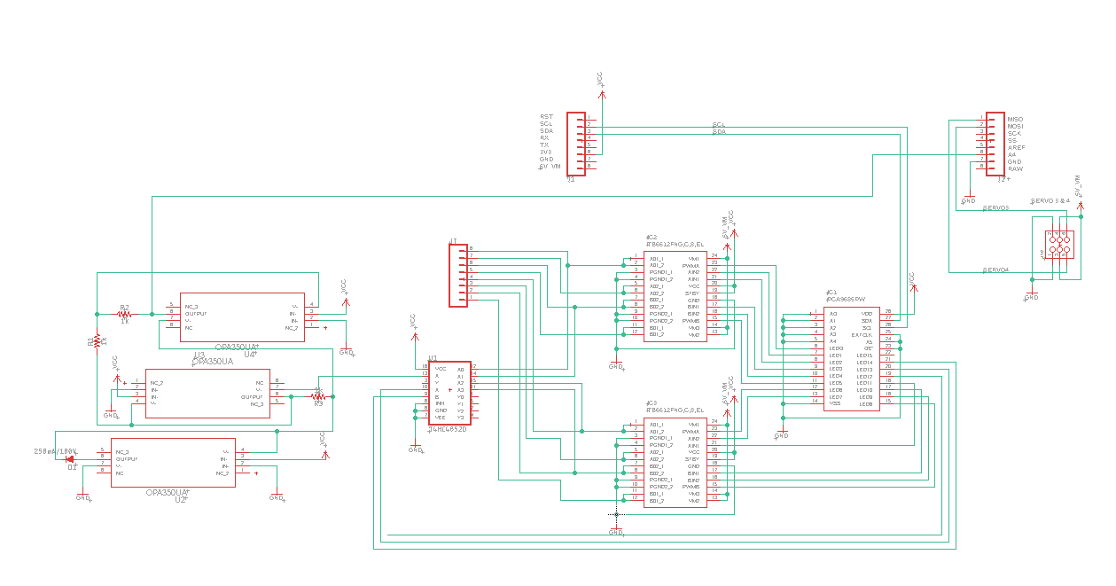
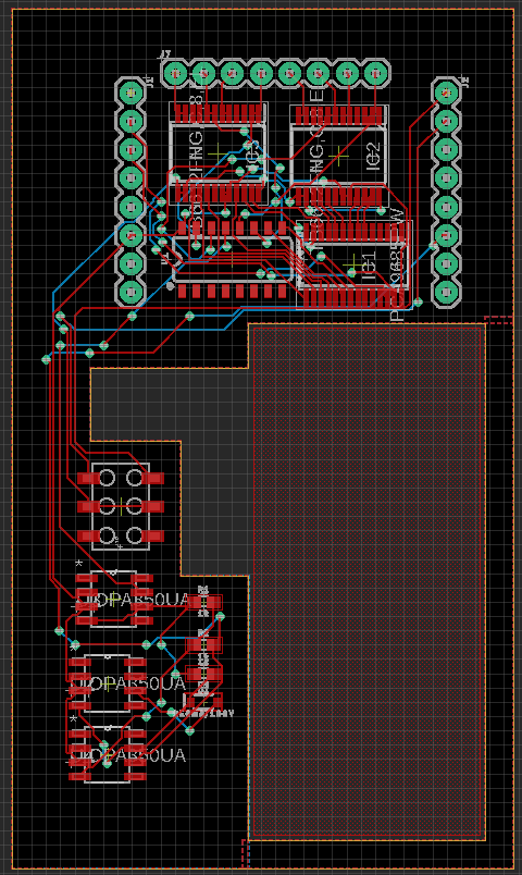
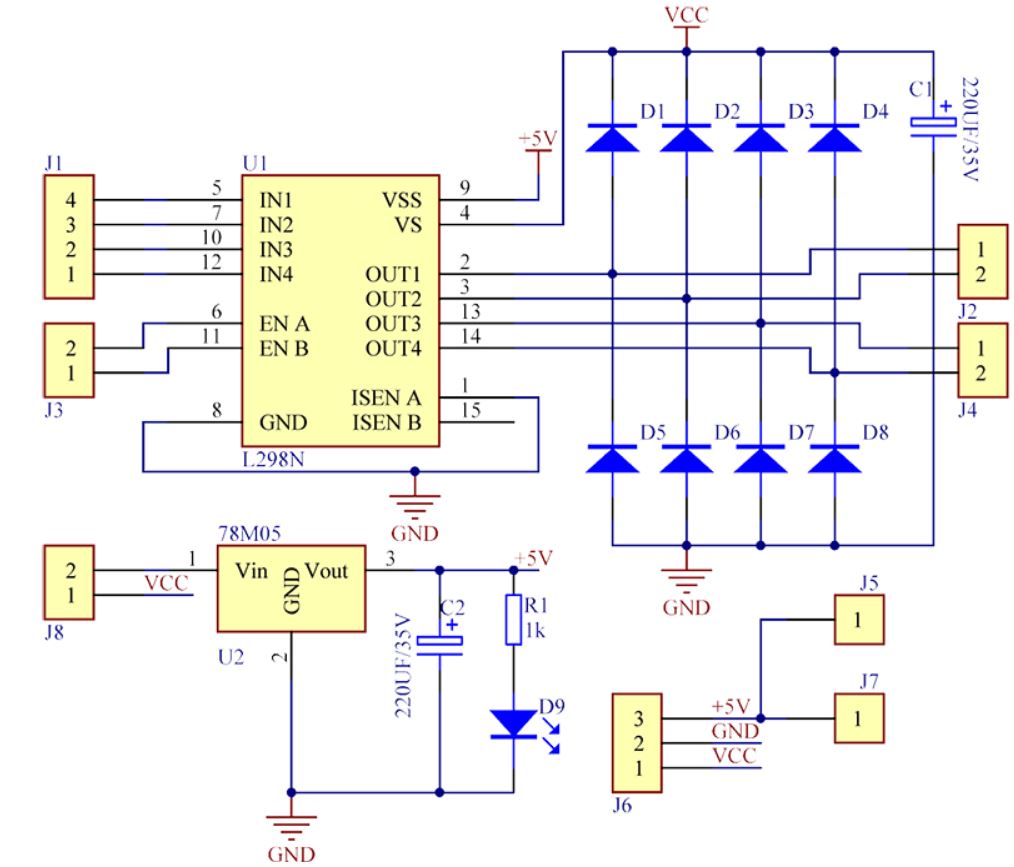
For the back EMF PCB we needed to send the motor data to the A4 pin which is one of the 3DoT’s ADC pins. To make more space on the board we added headers on the top for our four motors, replacing the larger jst motor headers. We also moved the cutout slightly higher up to give us more space to access the servo and motor headers on the 3DoT. Since we only had access to one ADC pin and we wanted to get readings from four motors we used a multiplexer connected to the PWM driver to switch between readings. Since our ADC was not able to get negative results we added in a full wave rectifier to the output of the multiplexer before the results were sent to the ADC. This allows us to determine the RPM of the motors when they are travelling in the opposite direction and to use our software to determine the direction. The original board that we were given to use with Sojourner is the motor driver shield design by Jaap from AoSA. This shield’s IC parts were reorganized and placed into the top part of the PCB to make more space for the full wave rectifier.
[/av_textblock]
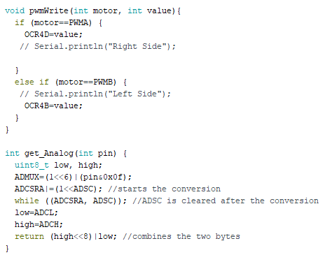
[av_heading tag=’h2′ padding=’10’ heading=’Firmware’ color=” style=” custom_font=” size=” subheading_active=” subheading_size=’15’ custom_class=” admin_preview_bg=” av-desktop-hide=” av-medium-hide=” av-small-hide=” av-mini-hide=” av-medium-font-size-title=” av-small-font-size-title=” av-mini-font-size-title=” av-medium-font-size=” av-small-font-size=” av-mini-font-size=”][/av_heading]
[av_textblock size=” font_color=” color=” av-medium-font-size=” av-small-font-size=” av-mini-font-size=” admin_preview_bg=”]
#include
#include <avr/io.h>
#include “3DoTConfig.h”
//#include “Averager.h”
uint16_t sample;
//average backEMF(sensor,8); //10 is the buffer depth and is adjustable
void setup() {
// put your setup code here, to run once:
init3DoT();
digitalWrite(AIN1,LOW);
digitalWrite(AIN2,HIGH);
pwmWrite(PWMA,100);
initADC();
}
void loop() {
// put your main code here, to run repeatedly:
//FSM measure back EMF
static int state=0;
const uint32_t timeDelay = 50;
switch(state) {
case 0:
//can also try the attachinterrupt method
if(TCNT4 == OCR4D){
state=1;
}
break;
case 1:
static uint32_t endOfDelay=micros()+ timeDelay;
if (micros() > endOfDelay){
state=2;
uint16_t sample=get_Analog(A3);
//grab ADC sample
}
break;
case 2:
Serial.println(sample);
//can also add running averager
/*
* if (firstRun==1){grab 8 samples if still doing running averager}
* sample=analogRead(A3) or readSensor(A3)
*/
state=3;
break;
case 3:
//getAvg();
//Serial.println(sample);
state=0;
break;
}
}
void pwmWrite(int motor, int value){
if (motor==PWMA) {
OCR4D=value;
// Serial.println(“Right Side”);
}
else if (motor==PWMB) {
// Serial.println(“Left Side”);
OCR4B=value;
}
}
int get_Analog(int pin) {
uint8_t low, high;
ADMUX=(1<<6)|(pin&0x0f);
ADCSRA|=(1<<ADSC); //starts the conversion
while ((ADCSRA, ADSC)); //ADSC is cleared after the conversion
low=ADCL;
high=ADCH;
return (high<<8)|low; //combines the two bytes
}
[/av_textblock]
[av_textblock size=” font_color=” color=” av-medium-font-size=” av-small-font-size=” av-mini-font-size=” admin_preview_bg=”]
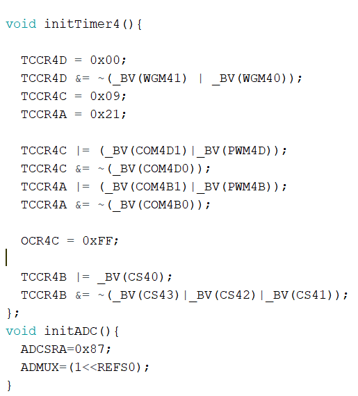
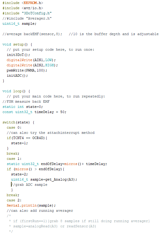
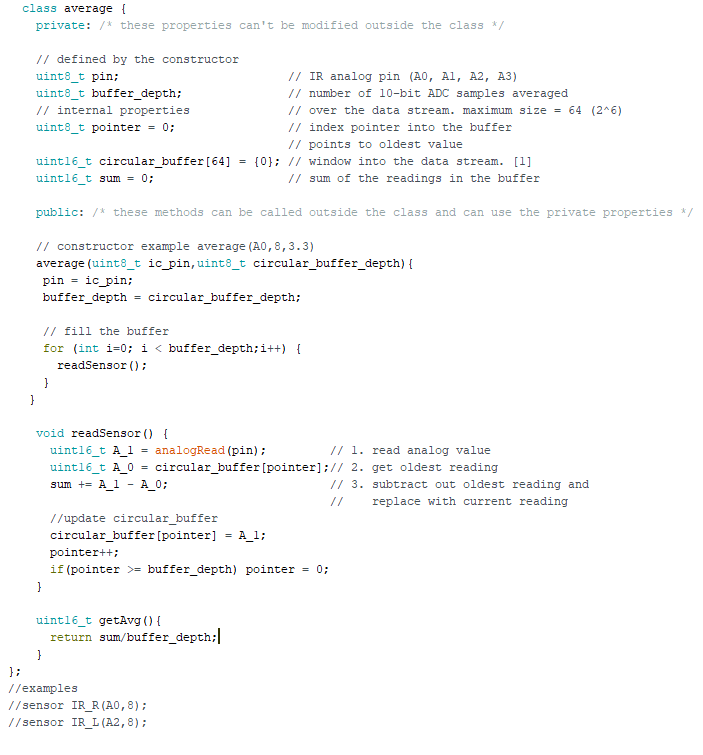
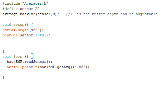
Our firmware for this project involved creating code for testing the back emf circuit. To do this we went through multiple iterations on an FSM. The goal of this code was to be able to grab ADC readings within a narrow length of time to avoid damaging the ADC from an early reading during a voltage and before the next PWM cycle started. For this we also created a class based running averager to implement at the end for our RPM readings. For our initializations we used the timer and adc registers to avoid using arduino’s prewritten functions that were too slow for our project. For the control of Sojourner we created command handlers to interact with the Arxrobot app using the Arxterra libraries.
[/av_textblock]
[av_heading tag=’h1′ padding=’10’ heading=’Mechanical/Hardware Design’ color=” style=” custom_font=” size=” subheading_active=” subheading_size=’15’ custom_class=” admin_preview_bg=” av-desktop-hide=” av-medium-hide=” av-small-hide=” av-mini-hide=” av-medium-font-size-title=” av-small-font-size-title=” av-mini-font-size-title=” av-medium-font-size=” av-small-font-size=” av-mini-font-size=”][/av_heading]
[av_image src=’https://www.arxterra.com/wp-content/uploads/2020/05/Fusion1.png’ attachment=’162622′ attachment_size=’full’ align=’center’ styling=” hover=” link=” target=” caption=” font_size=” appearance=” overlay_opacity=’0.4′ overlay_color=’#000000′ overlay_text_color=’#ffffff’ animation=’no-animation’ admin_preview_bg=”][/av_image]
[av_textblock size=” font_color=” color=” av-medium-font-size=” av-small-font-size=” av-mini-font-size=” admin_preview_bg=”]
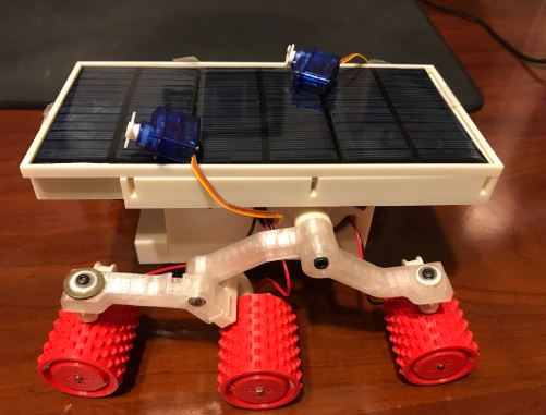
Figure 19 – Sojourner Fusion 360 View
[/av_textblock]
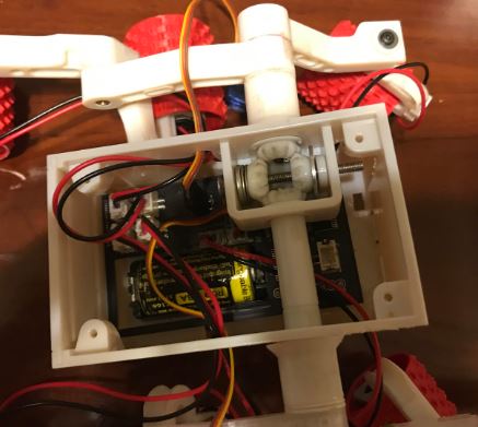
[av_image src=’https://www.arxterra.com/wp-content/uploads/2020/05/sojourner-1.jpg’ attachment=’162661′ attachment_size=’full’ align=’center’ styling=” hover=” link=” target=” caption=” font_size=” appearance=” overlay_opacity=’0.4′ overlay_color=’#000000′ overlay_text_color=’#ffffff’ animation=’no-animation’ admin_preview_bg=”][/av_image]
[av_textblock size=” font_color=” color=” av-medium-font-size=” av-small-font-size=” av-mini-font-size=” admin_preview_bg=”]
Figure 20 – Completed Sojourner
[/av_textblock]
[av_textblock size=” font_color=” color=” av-medium-font-size=” av-small-font-size=” av-mini-font-size=” admin_preview_bg=”]
The four parts that split Sojourner into are the solar tray, phone holder, main chasis, and rocker bogie. The solar tray holds the solar panels in the proper position to provide them with sunlight. This part also provides a cover for the phone holder. The phone holder has clips to keep the phone in the correct position to get video that can be displayed to the control panel. It also has space to include a periscope to get better vision. This part is screwed onto the main chasis to cover it and position the solar tray. The main chasis holds the 3DoT microcontroller and has holes for the wires to connect to the wheels and servos. It holds the gearbox which keeps the two rocker bogies connected to the main chasis and moving in sync. The rocker bogie keeps are wheels in place and has mounts to connect the servos to the motors for steering. It is designed to help Sojourner overcome difficult terrain. These are the four main parts that comprise our 3D model.
[/av_textblock]
[av_heading tag=’h1′ padding=’10’ heading=’Verification & Validation Test Plan’ color=” style=” custom_font=” size=” subheading_active=” subheading_size=’15’ custom_class=” admin_preview_bg=” av-desktop-hide=” av-medium-hide=” av-small-hide=” av-mini-hide=” av-medium-font-size-title=” av-small-font-size-title=” av-mini-font-size-title=” av-medium-font-size=” av-small-font-size=” av-mini-font-size=”][/av_heading]
[av_textblock size=” font_color=” color=” av-medium-font-size=” av-small-font-size=” av-mini-font-size=” admin_preview_bg=”]
Our verification plan has 5 test cases. Each one holds the 5 portions of our project that being: Basic Operations, Mission Operation, Sojourner Build, Logistics and Research. Basic operations verifies Sojourner’s Telemetry and basic functions of turning the motors with the ArxRobot App. Originally planned to be demonstrated, many of the requirements here had to be pushed to video due to the failures (wearing down) of the 3D printed parts and no access/time to reassemble Sojourner before verification. Due to the failure of the 3D printed parts (what we were thinking to be the material PETG, being too soft for continual use), the mission operation requirements, initially intended for demonstration needed to be cut as well.
For Sojourner’s build instructions, we found it easy to be done through inspection to make sure Sojourner was safe and accessible for the intended audience of children. Research verification was included to discuss the need of the sensorless encoding and its implementation. The verification plan can be found here.
[/av_textblock]
[av_heading tag=’h1′ padding=’10’ heading=’Concluding Thoughts and Future Work’ color=” style=” custom_font=” size=” subheading_active=” subheading_size=’15’ custom_class=” admin_preview_bg=” av-desktop-hide=” av-medium-hide=” av-small-hide=” av-mini-hide=” av-medium-font-size-title=” av-small-font-size-title=” av-mini-font-size-title=” av-medium-font-size=” av-small-font-size=” av-mini-font-size=”][/av_heading]
[av_textblock size=” font_color=” color=” av-medium-font-size=” av-small-font-size=” av-mini-font-size=” admin_preview_bg=”]
Robert Pearson (Project Manager & Mechanical Engineer):
This semester, as a project manager, I was required to do a lot of quick thinking. As the entirety of the project changed from being on campus to being at home, calendars, scheduling, individual tasks and budget all needed to be changed. For example, when ordering parts to test out the commutator noise circuit in April, it was found that the fastest shipping could be done in 1-2 weeks; as the parts weren’t viewed as a priority. At this point I had to work with my group mates to plan “if we can’t be working on this, what task can be switched to at this time.”
A takeaway I would give to the next generation of Sojourner is to pinpoint the aspect of the project you want to focus and do well on. I believe our project turned out to be a sensorless rpm encoding generation #1 rather than a Sojourner generation #4. I would want the next iteration of Sojourner to continue working on the commutator noise circuit, as the circuit does work and is able to use ripple counting. I would say that the next step of this would be to properly write code similar to the Back EMF method. In turn one should be able to then implement the stacked PCB as intended onto the Back EMF/Motor Driver Shield.
Alex Dalton (Electronics & Control Engineer):
I would recommend to future teams working on coding for their 3DoT projects to read through the 3DoT libraries to understand what is going on behind the scenes. Doing this makes it much easier to make changes and add new code to the commands and telemetry of the robot. I also recommend always researching the ICs that you plan to use as the producers often have code to introduce how to use the components.
Another important aspect to approaching a new project is to decide what the most important parts of your project are. Groups should decide to focus more on research or building from the very beginning. I believe that our team was off to a very good start at the beginning of the semester, but due to restrictions placed upon us due to the lockdown orders and the loss of access to the school’s resources we were not able to fully develop the class as much as we would want.
David Garcia (Mission, System & Test Engineer):
Looking back at this semester, there were some mistakes that could have been easily avoided. Attempting to order a PCB for the first validation test stands out as a big mistake. The largest misstep for our team was to start in two directions, one research and the design based and never get to bring those two paths together as closely as we would have. I think it would have been much better for us to have started as a purely research and experimentation team and work in design only once we got some experimental results.
I can not more strongly recommend not taking this class during a worldwide pandemic. Cooperation is difficult when your teammates are a possible source of death and destruction.
[/av_textblock]
[av_heading tag=’h1′ padding=’10’ heading=’References/Resources’ color=” style=” custom_font=” size=” subheading_active=” subheading_size=’15’ custom_class=” admin_preview_bg=” av-desktop-hide=” av-medium-hide=” av-small-hide=” av-mini-hide=” av-medium-font-size-title=” av-small-font-size-title=” av-mini-font-size-title=” av-medium-font-size=” av-small-font-size=” av-mini-font-size=”][/av_heading]
[av_textblock size=” font_color=” color=” av-medium-font-size=” av-small-font-size=” av-mini-font-size=” admin_preview_bg=”]
- Project Video
- Design Review
- Initial Research Presentation
- Burndown
- Verification and Validation Plan
- Solidworks Files
- Version 2 Presentation
- EagleCAD files
- Firmware
- Bill of Materials
- Mechanical BOM
- Sojourner Spring 2020 Schedule
[/av_textblock]
[/av_one_full]