ATTEMPT 1 OF INVERSE KINEMATICS USING MATLAB
By: Grace Hutchinson
Editors Note: This article is actually about modeling a robotic arm using Forward Kinematics in Matlab.
With each new iteration of the arm design, the length of the arm led to the need of an inverse kinematics study. Inverse kinematics is the process of using joints and angles to calculate how something will move, in this case we wanted to know how the Build-A-Block arm would move. By calculating the inverse kinematics we were able to map out and mimic how the arm would behave.
Figure 1 is a diagram to show how the MATLAB code was modeled. The solid blue line represents the first part of the arm between two joints with the dotted blue line showing the range of movement with the angle 1 limitations. The solid red line represents the second part of the arm after the middle joint with the dotted red line showing the range of movement with the angle 2 limitations.

Figure 1. Part 1 Inverse Kinematics Joints Diagram
Below are the inverse kinematic equations to solve using the diagram in Figure 1. In order to find the angles you must have the arm lengths and the x/y coordinates.
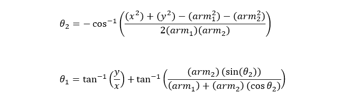
Figure 2. Inverse Kinematic Angle Equations
The MATLAB code below was used in the inverse kinematic calculations, this was created with the help of Mathworks.
clear, clc
arm1 = 90;  % length of V1 arm 1 before joint in mm
arm2 = 140; % length of V1 arm 2 before joint in mm

arm3 = 140; % length of V2 arm 1 before joint in mm
arm4 = 190; % length of V2 arm 2 before joint in mm

angle1 = 0:0.1:pi/4; % all possible angles for arm 1
angle2 = -pi:0.1:0;  % all possible angled for arm 2

[ang1,ang2] = meshgrid(angle1,angle2); % grid of angles1 and angles2

x1 = arm1*cos(ang1)+arm2*cos(ang1+ang2); % V1 x coordinates
y1 = arm1*sin(ang1)+arm2*sin(ang1+ang2); % V1 y coordinates

x2 = arm3*cos(ang1)+arm4*cos(ang1+ang2); % V2 x coordinates
y2 = arm3*sin(ang1)+arm4*sin(ang1+ang2); % V2 y coordinates

figure()
plot(x1, y1,'r.');
grid on
xlabel('Distance in Millimeters')
ylabel('Distance in Millimeters')
title('Coordinates for V1 Arm Using Forward Kinematics')

figure()
plot(x2, y2,'b.');
xlabel('Distance in Millimeters')
ylabel('Distance in Millimeters')
title('Coordinates for V2 Arm Using Forward Kinematics')
grid on
In Figure 3 the graph displays the inverse kinematics for the V1 arm, when the length of the arm segments at the joint are 90 mm and 140 mm. The red dots represent the motion of the arm reach in mm for the x and y axis. Here we can observe that the arm can only reach up to 143.6 mm (without the Golaith and attachment piece) and 212.2 mm with the entire Build-A-Block robot built. The arm can also reach down to -139.9 mm, which is necessary, as the robot arm stacked on the Golaith base will need to be able to reach down for the Jenga blocks.
This height and motion was good enough for a V1 demo to understand the movement, however we quickly realized that the arm would not be long enough to reach higher than a fully built Jenga tower of 224 mm.
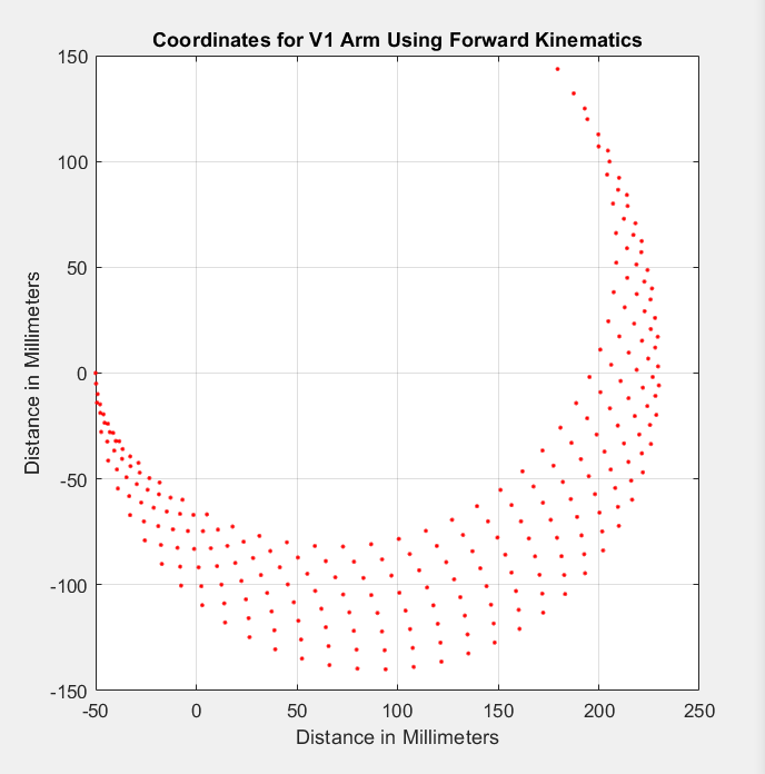
Figure 3. Part 1 V1 Inverse Kinematics
In Figure 4 the graph displays the inverse kinematics for the V2 arm, when the length of the arm segments at the joint are 140 mm and 190 mm (a 50 mm increase from the V1 design). The blue dots represent the motion of the arm reach in mm for the x and y axis. Here we can observe that the arm is able to reach up to 206.4 mm (without the Golaith and attachment piece) and 275 mm with the entire Build-A-Block robot built. The arm can also reach down to -189.9 mm, which again is necessary, as the robot arm stacked on the Golaith base will need to be able to reach down lower for the Jenga blocks.
This height and motion for V2 allows Build-A-Block the ability to build the full height Jenga tower of 224 mm, as well as extra length to play the game of Jenga and build the tower up higher. We will keep the V2 arm length the same for V3, and no changes will be made to the joint connections as the inverse kinematics is at the standard necessary for the robot to function.
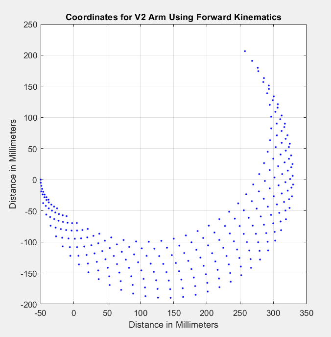
Figure 4. Part 1 V2 Inverse Kinematics
ATTEMPT 2 OF INVERSE KINEMATICS USING MATLAB
In Part 1 we were trying to model the inverse kinematics of the robotic arm, however not all of the motion was being calculated. The robotic arm model we are using has 3 sections to the arm, section 1 of the arm represents the “bicep” and is attached to the base right before the “elbow” joint, section 2 of the arm is also attached to the base and works as a “shoulder”, and section 3 of the arm represents the “forearm” that is connected right after the “elbow” joint. In Part 1 we modeled the arm using just the bicep and forearm pieces, however we did not take into account the motion coming from the shoulder piece.
In Part 2 we attempted to alter the code so that all three sections of the arm were modeled in the kinematics calculations. This was done by have 4 angles in total:
- Angle 1 : All possible angles of bicep section in motion
- Angle 2: All possible angles of forearm section in motion when only the bicep is in motion
- Angle 3: All possible angles of shoulder section in motion
- Angle 4: All possible angles of forearm section in motion when only the shoulder is in motion
By have 4 angles we were able to model angle 2 to be dependent on angle 1, and angle 4 to be dependent on angle 3 without effecting the other pair of angles. The motion was divided into 2 separate inverse kinematic plots and combined to show the difference and the overlap. Below in Figure _ is the diagram that the code is based on.
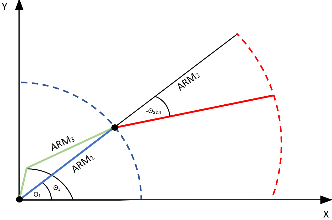
Figure 4. Part 2 Inverse Kinematics Joints Diagram
clear, clc
arm1 = 90;   % length of V1 arm 1 "bicep" in mm
arm2 = 140;  % length of V1 arm 2 "forearm" in mm
arm3 = 90;   % length of V1 arm 3 "shoulder" in mm

arm11 = 140; % length of V2 arm 1 "bicep" in mm
arm22 = 190; % length of V2 arm 2 "forearm" in mm
arm33 = 140; % length of V2 arm 3 "shoulder" in mm

angle1 = 0:.1:pi/4;         % all possible angles for arm 1
angle2 = -5*pi/6:.1:0;      % all possible angles for arm 2 w/ arm 1
angle3 = 0:.09:7*pi/18;     % all possible angles for arm 3
angle4 = -5*pi/6:.09:-pi/3; % all possible angles for arm 2 w/ arm 3

[ang1,ang2] = meshgrid(angle1, angle2);
[ang3,ang4] = meshgrid(angle3, angle4);

x1 = arm1*cos(ang1) + arm2*cos(ang1 + ang2);   % V1 x coordinates pt.1
y1 = arm1*sin(ang1) + arm2*sin(ang1 + ang2);   % V1 y coordinates pt.1

x2 = arm3*cos(ang3) + arm2*cos(ang3 + ang4);   % V1 x coordinates pt.2
y2 = arm3*sin(ang3) + arm2*sin(ang3 +ang4);    % V1 y coordinates pt.2

x3 = arm11*cos(ang1) + arm22*cos(ang1 + ang2); % V2 x coordinates pt.1
y3 = arm11*sin(ang1) + arm22*sin(ang1 + ang2); % V2 y coordinates pt.1

x4 = arm33*cos(ang3) + arm22*cos(ang3 + ang4); % V2 x coordinates pt.2
y4 = arm33*sin(ang3) + arm22*sin(ang3 + ang4); % V2 y coordinates pt.2

figure()
plot(x1, y1,'r.');
hold on
grid on
xlabel('Distance in Millimeters')
ylabel('Distance in Millimeters')
title('Coordinates for V1 Arm Using Forward Kinematics')
plot(x2, y2,'m.');
grid on
hold off

figure()
plot(x3, y3,'b.');
hold on
grid on
xlabel('Distance in Millimeters')
ylabel('Distance in Millimeters')
title('Coordinates for V2 Arm Using Forward Kinematics')
plot(x4, y4,'c.');
grid on
hold off
In Figure 5 the kinematics for Part 2 of V1 are modeled, with the red dots representing the work done in Part 1. The pink dots represent the results of the added code, thus showing how the inclusion of the shoulder section of the arm greatly increases the potential motion. The arm still reaches up and down to the same levels of 146.2 mm and -139.8 mm, however now it can also reach closer in front. There are still slight errors, as can be seen in the cutoff of the pink dots when reach up to 94.34 mm, therefore more work still needs to be done to improve upon the code in order to model the full extent of the inverse kinematics for the robotic arm.
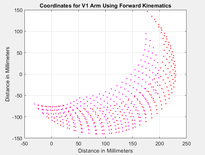
Figure 5. Part 2 V1 Inverse Kinematics
In Figure 6 the kinematics for Part 2 of V2 are modeled, with the blue dots representing the work done in Part 1. The light blue dots represent the results of the added code, thus showing how the inclusion of the shoulder section of the arm greatly increases the potential motion. The arm still reaches up and down to the same levels of 210 mm and -189.7 mm, however, now it can also reach closer in front. There are still slight errors, as can be seen in the cutoff of the light blue dots when reaching up to 144.5 mm, therefore more work still needs to be done to improve upon the code in order to model the full extent of the inverse kinematics for the robotic arm.
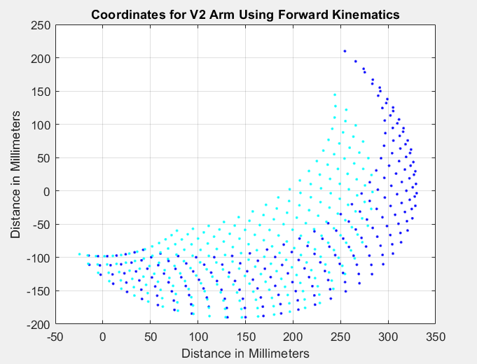
Figure 6. Part 2 V2 Inverse Kinematics
ATTEMPT 3 OF INVERSE KINEMATICS USING MATLAB
In Part 2 we were trying to model the inverse kinematics of the robotic arm with more motion implemented. The robotic arm model were using had 3 sections to the arm, section 1 of the arm represented the “bicep” and is attached to the base right before the “elbow” joint, section 2 of the arm was also attached to the base and worked as a “shoulder”, and section 3 of the arm represented the “forearm” that was connected right after the “elbow” joint. In Part 3 we decided to keep all angles and arm sections the same, as it was very close to representing the arm movement. The only issue was changing the length of one of the arm pieces.
In Part 3 we attempted to alter the code so that all three sections of the arm were modeled in the kinematics calculations. This was done by altering arm length:
- Arm 1: “Bicep” remained the same length
- Arm 2: “Forearm” remained the same length
- Arm 3: “Shoulder” length was increased to model how it grabs the “forearm” from further back

Figure 7. Part 3 Inverse Kinematics Joints
Below is the updated code:
arm111 = 90; % length of V1 arm 1 "bicep" in mm
arm222 = 140; % length of V1 arm 2 "forearm" in mm
arm333 = 120; % length of V1 arm 3 "shoulder" in mm

arm1111 = 140; % length of V2 arm 1 "bicep" in mm
arm2222 = 190; % length of V2 arm 2 "forearm" in mm
arm3333 = 180; % length of V2 arm 3 "shoulder" in mm

angle111 = 0:.1:pi/4; % all possible angles for arm 1
angle222 = -5*pi/6:.1:0; % all possible angles for arm 2 w/ arm 1
angle333 = 0:.09:7*pi/18; % all possible angles for arm 3
angle444 = -5*pi/6:.09:-pi/3; % all possible angles for arm 2 w/ arm 3

[ang111,ang222] = meshgrid(angle111, angle222);
[ang333,ang444] = meshgrid(angle333, angle444);

x111 = arm111*cos(ang111) + arm222*cos(ang111 + ang222); % V1 x coordinates pt.1
y111 = arm111*sin(ang111) + arm222*sin(ang111 + ang222); % V1 y coordinates pt.1

x222 = arm333*cos(ang333) + arm222*cos(ang333 + ang444); % V1 x coordinates pt.2
y222 = arm333*sin(ang333) + arm222*sin(ang333 + ang444); % V1 y coordinates pt.2

x333 = arm1111*cos(ang111) + arm2222*cos(ang111 + ang222); % V2 x coordinates pt.1
y333 = arm1111*sin(ang111) + arm2222*sin(ang111 + ang222); % V2 y coordinates pt.1

x444 = arm3333*cos(ang333) + arm2222*cos(ang333 + ang444); % V2 x coordinates pt.2
y444 = arm3333*sin(ang333) + arm2222*sin(ang333 + ang444); % V2 y coordinates pt.2

figure()
plot(x1, y1,'r.');
hold on
grid on
xlabel('Distance in Millimeters')
ylabel('Distance in Millimeters')
title('Coordinates for V1 Arm Using Forward Kinematics')

plot(x222, y222,'m.');
hold off

figure()
plot(x3, y3,'b.');
hold on
grid on
xlabel('Distance in Millimeters')
ylabel('Distance in Millimeters')
title('Coordinates for V2 Arm Using Forward Kinematics')

plot(x444, y444,'c.');
hold off
Below in Figures 8 & 9 are the updated inverse kinematics for V1 and V2 of the arm. The overlap of light and dark blue/red points compares the Part 1 data with the improved Part 3 data. The arm still reaches down and up the same as found in Part 1, however now the forward reach has increased.
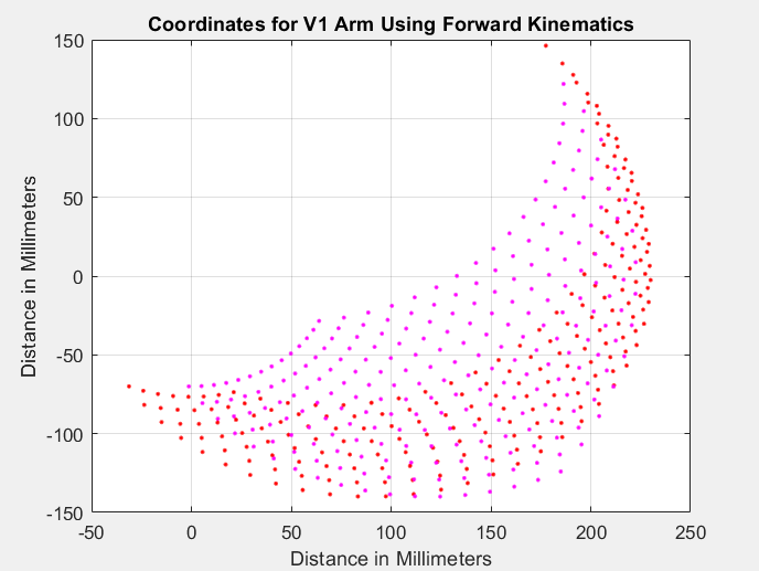
Figure 8. Part 3 V1 Inverse Kinematics
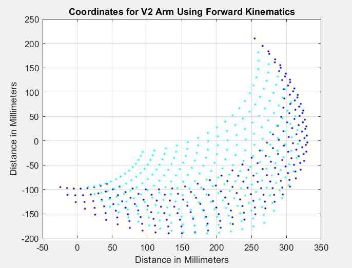
Figure 9. Part 3 V2 Inverse Kinematics